
 The "Barèges" CCD Spectrograph
Contributions: A. & S. Rondi, C. Buil / S. Dearden (translation)
|
|
|
The
idea of the Barèges spectrograph was created in a splendid flat at the
famous Pyrenean ski resort that bears its name during one glorious winters
day in 2003.
You
will find similar spectrograph designs on the Spectros
Connection
|
|
|
This page describes the step-by-step
construction of the Barèges spectrograph and also provides some instructions
and guidance in setting up and initial operation.
|
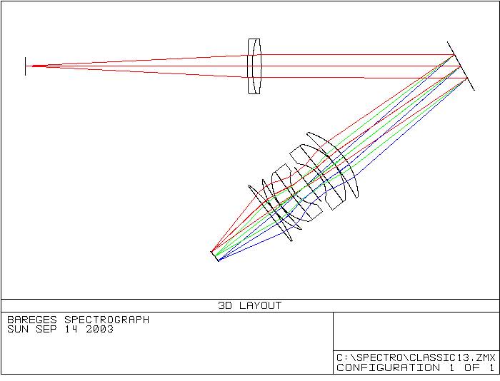
Optical CharacteristicsAn optical
schematic of the Barèges Spectrograph is shown below. |
 |
Main Characteristics
|
 |
 |
 |
|
Cut out two identical shapes from 4mm aluminium sheet as shown. Some of the holes to be drilled are in exactly the same positions on both sheets, although others are not, so care must be taken with your drilling! Take care also to countersink the holes on the correct side of the sheets. Countersinking the holes can be avoided for those wishing to use flat-head metal screws in place of the countersunk type. Note that it is also possible to use thinner gauge aluminium sheet whilst still maintaining good stiffness and rigidity and having the advantage of reducing the total weight of the spectrograph. If this is the case then the appropriate length of flat-head screws must be used.
|
A large format (400x600) gif image of Part P2 can be found by clicking 2Dbase, or by using the Varicad application described above.
|
 |
Support plate
S2 is cut out from a piece of aluminium or Dural sheet, and will be used
to support all the entrance slit components. Adjustment screws Ft5 and Ft6 are made from brass. Two tensioning springs (not shown) wrap around rod Ft4, one connecting the side L4 and stage Ft1 and the other connecting L3 and Ft2.
|
 |
The plate S2 is drilled with a central hole of 35mm diameter, and all holes are tapped to a depth of 12 mm with an M4 thread. |
 |
Translation
stages Ft1 and Ft2 are made from 8mm thick aluminium and drilled as indicated
in the drawing opposite. Special care needs to be taken during machining
the shape to achieve smooth transverse movement with no play.
|
 |
The two side
panels L3 and L4 are drilled with 5mm diameter non-piercing holes. They
are used to locate rods Ft3 and Ft4. L3 and L4 are cut from 3mm aluminium sheet. |
 |
The last thing that remains to be done is to assemble these, our first, pieces |
 |
The metal entrance plate is cut from 8mm aluminium sheet. Note the two 6mm drill holes for fixing the telescope adaptor (part T2). The central hole is 35mm in diameter, for example. As for all S-panel components, all holes are tapped to receive M4 screws. |
 |
The dimension
for part T2 is indicative only, since it is up to each amateur either
to machine his or her own adapter or buy one commercially available for
their telescope. |
 |
The part opposite is an adaptor for right-angle observation with a Newtonian reflector with an eyepiece holder of 53mm diameter (Clavé type). It is attached to the base plate of the spectrograph with 3 screws (not shown). Here again it is left to each amateur to adapt the design to his particular instrument. More often than not, it is better to design for both types of possible connections. |
 |
Shown here is the assembly at the end of stage 3... |
 |
The collimator support plate (S3), just like all the other S components, is made from 8mm Al sheet. Note the 6mm above the collimator lens hole this will be used to attach an order-sorting filter.
|
 |
The achromat lens used as the collimator is a doublet of focal length 125mm and diameter 30mm (obtainable from Edmund Optics, Ref. No. A45-217). When positioned at 125mm from the slit, rays of light that are focused on the slit will exit the collimator as a parallel beam which then goes on to the grating. Part F3, the ring for the order-sorting filter, can be installed at this point, prior to adding the support and filter (next stage). The two parts are in PVC tubing 32x3. |
 |
The two PVC parts are glued to the S2 and S3 plates, as shown on the exploded view. C1 tube can the slide inside for focusing. |
 |
The completed collimator group. |
 |
The order filter needs to be an orange or red long-pass variety. Standard photographic filters can be used perfectly well. The minimum diameter should be at least equal to the diameter of the collimator (30mm in this case). The filter is mounted in a small aluminium support (part F1) that is rotated by rod F4. This rod, 76mm long and 5mm in diameter, is made of plastic composite (for lightness and strength) and is glued to F1 as shown. F4 is inserted in brass tube F2 (6mm o.d., 5mm i.d.), 50mm in length. F2 is then attached (by Araldite) onto panel S3, flush with it on the slit side and extending on the filter side. A tensioning spring (not shown) must be attached around the tube F2 and pulling on S3 and F5 to take up any play. Brass knob F5 pushes onto F2 and is locked by a small tightening screw
|
 |
F1 Shown opposite is part F1, made from aluminium. Some handy work with a file should achieve the right size and shape. |
 |
In this drawing the order-sorting filter can be seen in the light beam (where it will be used to separate diffraction order 1 from higher orders). It can also be seen in the out position in wire-frame rendering. |
 |
The grating
mount must permit fine adjustments to the angle of incidence of parallel
rays from the collimator. In this way it allows us to examine dispersed light from the grating
as a function of wavelength. |
 |
Part R2 is made of aluminium. It is to be screwed (or glued) onto the spectrograph top cover P1 through which the central axis rod R9 passes. Rod R9 has 19 x 6 groove to accept a ball bearing (refer to drawing). The grating support plate should not present any particular problem in construction. Note that the two insertion holes for threaded rods R10 and R10 off-axis by about 4.9mm, allowing the grating to rotate around its optical plane. The insertion holes are tapped with M$ taps to receive the above threaded rods. Lock the rods in place with glue. |
 |
The large aluminium rotation arm R3 has a groove on the side with a 6mm hole to fasten to axis rod R9 by screw R13. A central hole is drilled and M4 tapped down rod R9 at one end to connect to rotation arm R3. At the other end R9 is threaded M6 on the outside for 8mm of its length to screw into the top grating mount R1. |
 |
Things are beginning to take shape! |
 |
The focusing
lens is a 35mm SLR camera objective. The one is a Nikon 50mm f/1.4 lens, but any
good quality SLR lens is suitable. |
 |
S4 - The machining of this straightforward part require no further comments, since it is by now familiar to us. |
 |
The objective lens itself (purple part) must not be mounted at this stage. It is added just before inserting the diffraction grating. |
 |
Several small parts still remain to be built. R4 and R5 are two easy pieces to make up. R4 is the guide plate for the grating rotation arm (R3) and plate R4 is attached to the top cover at the end of R3, where wavelength graduations in Angstrom units can be added. |
 |
Rear plate S5, situated behind the grating, has a 15mm diameter hole drilled through it. We shall see later that this is used to assist in focusing of the collimator lens. |
 |
Part T3 - This is a small eyepiece holder that can also be used to connect a Webcam and focusing optics. |
 |
Part M1 M1
is the support for a 75%/25% beam-splitter, of dimensions 25mm x 38mm
x 3mm (Edmund Optics Ref. No. A31-437) depending on whether the spectrograph
is used on the principal axis or in coudé mode. |
 |
It is also useful to add a turning knob on the outside of the spectrograph in order to conveniently rotate the beam-splitter. The knob is attached to the beam-splitter mount via a 4mm threaded rod
|
 |
Congratulations! Your first stellar spectrum is almost there! At this final stage the whole spectrograph now needs to be completely dismantled. Remove all optical components, cover the threaded rods with sellotape, and paint all interior surfaces matt black (spray can or brush). If you have made your spectrograph out of aluminium, thoroughly de-grease the metal surfaces prior to painting. It is also advisable to apply a coating of metal or plastic adhesion promoter prior to painting the interior of the instrument. Carefully remove all metal swarf from the outer surfaces of the spectrograph and lightly rub with emery paper. If you wish to paint the exterior, apply a metal primer as for the inside surface followed by spray can for metal to give a stippled effect (see your local DIY store).
|
 |
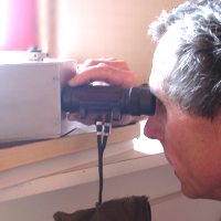 |
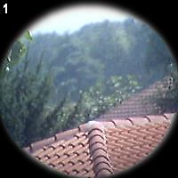
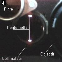
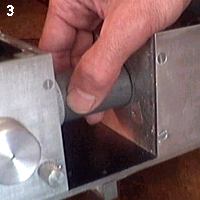
Slit Collimation:In order to
function correctly the slit must be located at the prime focus of the
telescope (see below how to do this). Diverging light from slit is then made parallel
by the collimator. Therefore the slit-collimator distance has to be equal
to the focal length of the collimator, in our case 150mm. To do this,
proceed as follows: With the aid of a small finder telescope, binoculars or a monocular lens set at infinity (1), aim through the hole in S5 to observe the two jaws of the slit at the opposite end of the spectrograph usually they will be out of focus (2). By carefully sliding (3) the PVC tube C1, fine adjustments can be made to the slit collimator distance to produce a sharp image (4). When this is achieved, fix C1 permanently in position by taping around C1 and C2 or C3. Avoid further changes to this setting. |
|
|
 |
|
 |
 |
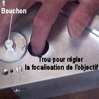
Focusing Lens and CCD:
Next, the correct
position for the CCD camera lens needs to be determined. This is attached
by screw V1 connecting, in this case, an Audine camera to the top cover
(P1) of the spectrograph. To do this, take some images of the slit with
the camera with the grating at the zero order position (90° to rays from
the collimator). Note that small changes in focus are necessary when changing diffraction orders and also when we move from the red to the blue in the spectrum. To achieve an acceptable degree of sharpness across the whole field, it is often important to turn the camera axis (use screw V1) by 1 or 2 degrees to compensate for residual chromatic aberration of the camera lens - an unavoidable phenomenon when we are using refractive optics (lenses) as opposed to reflective optics (mirrors). |
| 3 - spectre élargi d'un côté | 4 - spectre après shift correcteur | |

|
Beam-Splitter Positioning:This component rotates around its own axis by means of a knurled knob (1) that can be blocked in position by a locking ring (2). |
|
| 1 - image CCD (levres+etoile) | 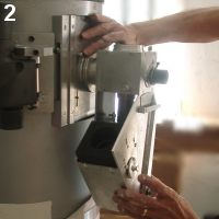 |
Placing the Slit at Telescope Prime Focus:The goal here
is to simultaneously produce a focused image of the slit (already achieved
during collimator adjustments) and a sharply focused image of a star on
the slit (1).
|
| 1 - image CCD (étoile au centre) | 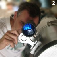 |
Aiming on a Star in Zero Order:In the usual way, ensure that the finder is in good alignment with the main telescope. Then centre a star on the cross hairs of the telescope finder and acquire an image in the middle of a CCD frame (1) by moving the main telescope. If necessary make readjustments to the finder position in order to re-centre the star image on the cross hairs. From this point on, do not touch this alignment. |
 |
2 - un spectre |
Focusing on
a 1st Order Spectrum:
Move to the
first order spectrum and fine tune the spectrum focus using the camera
focusing ring via the access hole in P1 as outlined above. All is now ready to acquire your very first stellar spectrum!
|
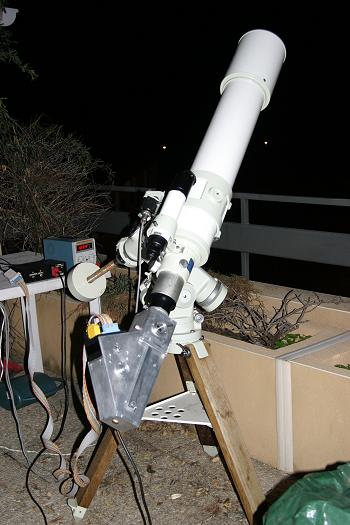 Le spectrograph in action!! (on 21st October 2003) |
Below is a spectrum of the star Alpheratz (a And). This is an overlay produced by superimposing ten 8-second exposures with a Takahashi FS-128 5 in. refractor and an Audine camera with a KAF-0401E chip. The full spectrum was obtained in two parts: for the visible region and the IR region (using the integrated blocking filter for the latter). Compositing was performed using IRIS software and spectral calibration with VisualSpec.
Spectrum of the Be star gamma-Cas, same scale as the spectrum above, a composite of fifteen 5-second exposures. Same telescope
Several other spectra obtained at Juillan during the testing and pre-qualification phase.


Zoom sur la raie H-alpha
|
As can be seen from the above results, the Barèges Spectrograph is capable of producing some excellent results. Amateurs looking into astronomical spectroscopy should be considering this kind of configuration, whether they are complete beginners or advanced observers. The instrument described is of the general-purpose medium resolution type that lends itself to a wide range of potential applications. |
The following links describe some other spectrographs with similar performance characteristics
- François Cochard spectrograph
Don't hesitate to contact us to add your home-made spectro to this list!
Many Thanks to Steve Dearden for this complete english translation of this page!!
![]()
