PROCESSING LHIRES SPECTRA
 Procedure using Iris / SPiris

French version
 

 1. INTRODUCTION

This paper presents a procedure to process LHIRES spectra using the software SPiris.  Basic use of the latter (or Iris) is a prerequisite to be able to read the tutorial.

The processing describes the conversion from  raw two-dimensional (2-D) spectra to the extraction of a calibrated spectral profile.

The example spectra (which can be downloaded) were acquired with the LHIRES III spectrograph mounted on an f/10 Celestron 11 telescope.  The gratings used are either  1200 lines / mm (dispersion 0344 / pixel), or 2400 lines / mm (dispersion  0115 A / pixel).  The camera is an Audine equipped with a Kodak KAF-0402ME CCD.  The entry slit is set to a width of 26 microns.  The observed region of the spectrum is centered on the Halpha line.  The resolution  is about R = 15000 with the 2400 lines / mm grating.  The observatory is in a heavily light polluted location, not far from the city of Toulouse (France).

 2. STARTING AND SETTING UP THE SOFTWARE

This tutorial is based on the software SPIris.  SPIris is a version of the program Iris and focuses on the processing of spectral data. Click here to download SPIris.

Start up the program SPIris then enter your working directory (ie, the directory containing the images to be processed).  For example, if the images are in the directory d: \ 130606 (directory name is the date of observation), open the dialog box Settings ... from the File menu and fill in as follows:

 The path to the working directory.

Please also indicate the type of image file, PIC for example.

Close the dialog box by clicking on OK.  You are now ready to deal with the spectra.

The spectra offered as an example were acquired on the night of 13 to 14 June 2006 with the LHIRES III spectrograph mounted on an f/10 Celestron 11 telescope.  The grating used is the 2400 lines / mm.  The camera is a Audine equipped with a Kodak KAF-0402ME CCD.  With this equipment, the average inverse spectral dispersion is 0115 A / pixel.  The entry slit is set to a width of 26 microns.  The resolution power is expected to be R = 15000.

 3. PROCESSING 2400 LINES/MM GRATING SPECTRA

 3.1. Processing the spectrum of the star Gamma Cas

We will process 7 spectra of the star Gamma Cas Be, made on the night of 10 to 11 June 2006.  The exposure time per image  is 180 seconds.

To download these spectra 7, click here (decompress the image files into your working directory).

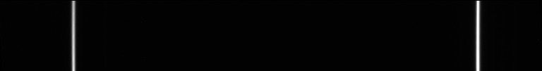
This is one of these raw spectra:

The file names of these spectra are generic "gcas-"  This means that the files are gcas-1, gcas-2, ..., gcas-7.

Note that the images are windowed 768 pixels x 100 pixels at acquisition.  This size is wide enough to record all the spectral information along the  horizontal axis.  The vertical height of 100 pixels is sufficient to give enough space either side of  the spectrum to measure the sky.  Of course, it also helps to save storage space and speed up processing.

We see in the raw images, the intense emission of the Halpha line at the centre and a few bright spots caused by thermal noise.  One can also see some narrow lines, caused by water vapour present in our own atmosphere.  These are known as telluric lines.  They are numerous and clear around the Halpha line.  They can disrupt the interpretation of the true spectrum of the star, but here, they are going to be our ally to enable us to calibrate the spectrum wavelength.  We must become accustomed to recognizing these lines.  One in particular.  It is located to the right of the Halpha line, on the red side, identified in the following image:

Note that the dispersion axis is exactly horizontal. Care has been taken to achieve that when adjusting the spectrograph (by rotating the CCD camera).

Immediately after observing Gamma Cas, we recorded a spectrum of the neon lamp.  Its name is gcas_neon-1.  Here is the spectrum:

Download this neon lamp spectrum here.

Note that the spectral lines are angled, which is a characteristic of the LHIRES III spectrograph.  There is nothing wrong with that.  We will use image processing to correct this.  To do this we must measure the angle of inclination of the lines from the vertical.  We will see how to do this later in this tutorial, but the result is the bank angle = -3.6 ° (also known as the angle of slant).  The command-line slant (or alternatively the dialogue box Slant of a 2D spectrum ... opened from the  Spectro menu) can straighten the lines, and can be used to determine the angle by making successive tests:

 > slant 50 -3.6

The first argument of this command is the vertical coordinate of the centre of the image (100 / 2).  The second parameter is the slant angle. Result:

We also need three  images to do the preprocessing: the offset (bias) image, the dark image (map of the thermal signal) and the flat-field image (uniformity of the light sensitivity).

 The offset image.

 The dark image

 The flat-field image

The corresponding image files are named in a natural way: offset, dark and flat.  To download these files, click here.

We need a fourth to complete the processing, a cosmetic file.  This file is optional, but it helps to treat difficult cases of hot pixels and the problem of column defects in the CCD.  This file, called cosme.lst, is a list in ASCII format which identifies such defects.  We will see later in the tutorial how to generate this file automatically.  For now, you can download it here (this version contains the 50 most intense hot pixels in the dark).

We now have everything to hand to deal with the Gamma Cas spectra (and all the other spectra acquired that night, and probably the following!).

SPIris has a powerful tool, specifically developed for the processing of LHIRES III spectra.  You must proceed in two stages.

Step1

Load the first spectrum of the sequence to be processed:

> load  gcas-1

 Another way is to use the Number command instead of the Load command.  The syntax is:

>number  gcas-

You must now select a rectangle in the spectrum using the mouse pointer:

To plot draw the rectangle, drag  the mouse while pressing the left mouse button.

What you need to know:

•  Draw the rectangle near the centre of the spectrum.  It may well not correspond to any  intense region.
•  The height of the rectangle should be such that it covers the full spectrum, including the less intense parts.  (To make the faint regions more visible, adjust  the  image threshold settings to increase the contrast.)  At the same time we must ensure the vertical dimension of the rectangle is not excessive.  It must be just enough to cover the all the spectrum with a small margin of only a few pixels (although the spectrum is tilted).
•  The width of rectange (horizontal axis) is not very critical.  Make it between 100 and 200 pixels long.

This rectangle is used by the software to identify the region of the image which contains the spectrum information, something that  the operator has to judge.

Step 2

Open the dialog box Treatment of LHIRES III spectra - 2400 from the Spectro menu:

This dialog box may appear impressive, but we must not be cowed!  Many of the fields are already pre-filled.  This is the case for the names of the standard preprocessing master images.  This is also the case for the generic name of the sequence of images to be processed and the number if you have taken the precaution of running the command number beforehand.

The only fields that you have to complete are:

•  The angle of slant or angle of inclination of the lines (here -3.6 °);
•  The position of the 6575 Angstrom water vapour line (here X = 468).

Leave everything else as it is.

Once you click OK, SPIris performs a very intensive calculation.  It does a complete preprocessing of the 7 spectra  (subtracting the offset, dark adjusted for the exposure time,  dividing by the flat-field, making cosmetic corrections), correcting the geometry (slant and tilt),  aligns the spectra , subtracts the sky background, makes a stack of the 7 images elliminating any artifacts (cosmic rays, electronic noise, ...),  bins  the 2-D spectrum into a 1-D spectrum (spectral profile) while optimizing the signal to noise, performs a precision wavelength calibration using the telluric lines in the spectrum and finally resamples using a fixed wavelength interval per pixel.

This processing takes only 3 to 5 seconds for your computer!

A single result is displayed on the screen:

This is the processed spectral profile of the star Gamma Cas (sum of individual spectra with all the calculations described previously).  To make it easier to see, the spectral profile is duplicated on 20 lines to form a pseudo  2-D spectrum.  This spectrum also has a linear dispersion, which was not the case for the raw spectra.  In this case, 1 pixel interval along the horizontal axis represents precisely a 0.1157 angstroms wavelength interval.

Information on the spectral calibration appears in the output window, which opens automatically:

There is the wavelength calibration error, and the wavelength of the first pixel of the image (here 6520.5 angstrom).  The coefficients of the second order polynomial  used to calibrate the spectrum wavelength are also given.  These factors are important for calibrating a spectrum in which the telluric H20 lines may not be visible (see example below).

A small note about the accuracy of the spectral calibration.  The residual error in the calibration (RMS) is 0.018 angstrom (The difference between the observed and calculated wavelengths using the polynomial).  This is a reasonably low error, it is possible to obtain a better result by using a star with a smoother spectral profile than Gamma Cas, for example, the star Altair.  Later in this tutorial, we will process a spectrum of this object.  Once the calibration coefficients have been obtained (a1 and a2 terms), they can be re-used to treat other stars without having to use telluric lines (we shall see this  in the following example, devoted to the star 64 Ser).

Currently, in a raw spectrum of Gamma Cas, the relationship between a number of pixel x and the corresponding wavelength is:

The coefficients a1 and a2 define the dispersion law for the spectrograph.  They are almost constant for a particular instrument, in a particular setup.  The term a0 defines spectral setting at the time of observation (that is the wavelength located at the extreme left of your spectrum).  If you move the spectrograph micrometer, this value is changed.  It is also modified as a result of mechanical flexing caused by differential loads on the spectrograph depending on the point observed in the sky.  In most cases, the work done by the software is to calculate the term a0. The terms a1 and a2 are assumed to be known (we will see that with the star 64 Ser).

SPIris wrote in the working directory three files corresponding to products level 0b, 0c and 1b.  The concept of level of product is important because it helps to break down the many stages of processing and the results obtained.  Intermediate steps are important to carry out checks, but also these intermediate products can be useful.  The spectral product levels are described here.

SPIris saves a level 0b image.  It is the sum of our individual 7 spectra .  The geometric corrections were carried out and the sky was subtracted.  This image is named 0b.pic in the example, but you may want to give it a different name (eg gcas_0b).

>load  0b

 The level 0b spectrum.

SPIris also saves a  level 0c spectrum, which is the 1-D version of the level 0b spectrum.  To do this, SPIris applied an optimal binning in terms of SNR.

>load  0c

 The level 0c spectrum.

Finally, the most important thing here. SPIris generated a level 1b product, which is the spectral profile of the star, calibrated in wavelength.  This profile is a simple two column ASCII file.  The first column contains the wavelengths in angstroms and in the second column the corresponding standardized intensity (the standard is the average intensity of the spectrum).  In our application, the file name is 1b.dat in the working directory (SPIris added  the extension .dat, to distinguish it from the image file).  Once again, you can use the name of your choice (for example gcas_1b.dat).

The contents of the level 1b file can be viewed and edited with a word processor, the output of SPIris / Iris can be displayed in the form of a graph in Excel or any other graphing program.  Above all it can be easily transported to spectral analysis software, as VisualSpec, to complete the processing and for further analysis (supplementary controls, correction for  the instrument response, normalization of the continuum, measurement of line equivalent line widths, etc.).

Here is an extract from the 1b.dat file:

To display the contents of the file in the form of a pseudo 2-D image, use the command

 >load  1b

 Representation of a level 1b product as an image (linear spectral dispersion).

 At this point you may get a clearer idea of the spectral profile by viewing it in graphical form:

>l_plot

Download the level 0b, 0c and 1b Gamma Cas products here.

 3.2. Processing the spectrum of the star 64 Ser

The star 64 Ser (HD175869) is a Be star of magnitude 5.57, thus significantly fainter than Gamma Cas.  The spectrum was obtained the same night and with the same instrumentation as for the observation of Gamma Cas.  We have taken15 spectra of the star, of 300 seconds exposure each.  Their generic name is "64ser-".

Confirm the number of images in the sequence from the console:

 >number  64ser-

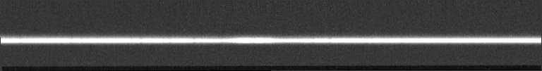
 Negative views of one of 15 raw images of 64 Ser.

We can use the same master images used for the Gamma Cas calibration.

Download the raw images of 64 Ser here.

Find the position of the 6574 A telluric H2O line:

The identification is much harder compared to Gamma Cas.  This is because Ser 64 is much less bright.  We can nevertheless find it, and we see that its position had not changed.  The other telluric lines are significantly less distinct, and you can guess that the software will have difficulty achieving a spectral calibration from them.  So we are not going to try to fit a polynomial calibration with the meagre information contained in the 64 Ser spectrum, but instead reuse the polynomial determined in the processing of Gamma Cas.

 Select the 64 Ser Spectrum with the mouse pointer:

Then open then the dialog processing Spectres LHIRES III - 2400  from the Spectro menu.  All fields are already filled in. You could, in principle, simply  click on OK. It could not be easier!  Do not do this, however.  We want to use the spectral calibration parameters found for the star Gamma Cas. We therefore ask SPIris not to recalculate.  To do  this, deselect the option  Calibration telluric lines (H20).  Make sure the position of  the 6575 A line is correct, as well as the right polynomial coefficients:

You can now click on OK.

There is an alternative method of calibration, if the telluric lines are completely invisible (either because the star is too weak or because the atmosphere is too dry, ...).

Load the neon image associated with the observation of 64 Ser:

>load  64ser_neon-1

With our inverse dispersion of 0.115 A / pixel only two neon lines are visible.  From left to right, they are located at the wavelengths  6532.8822 A and 6598.9529 A.  Locate the approximate position of the first line along the horizontal axis  using the mouse pointer.  You find roughly X = 105.  Download the spectrum 64ser_neon-1.

Reload the first spectrum of the Ser 64sequence, select the spectrum with the mouse, then open the dialog processing spectra LHIRES III - Spectro free from the spectro menu:

The box is impressive, but almost everything is already filled in.

You still have a little work to do:

•  Enter the wavelength of the left-most neon line chosen (6532.8822);
•  Enter the position of that line in the image 64ser_neon-1 (105);
•  Give it the filename of the neon  to use (64ser_neon-1);
•  Tell the software you are using the  2400 lines / mm grating.

Now click OK.  The processing to a calibrated spectral quality takes place in a few seconds.

SPIris processes  not only the spectrum of 64 Ser, but also that of your neon lamp.  It produces an intermediate file normally not accessible, but on an audit (and for education) you can see that processed spectrum (correction with the master images, geometric corrections), with:

> load @ @
> load @ @ @

Note that if you deselect the option Make a spectral calibration, SPIris does not generate the 0b and 0c level products.

Here is the calculated level 0b spectrum for Ser 64:

(Note the almost total absence of cosmetic defects)

And the level 0c spectrum

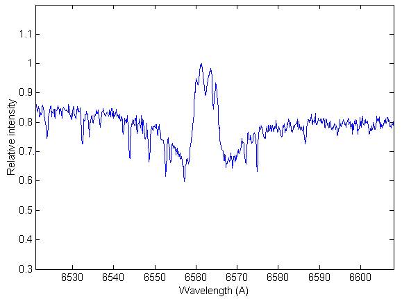
After a spell working with VisualSpec software, we get a level 2b product (telluric lines removed and normalised to the continuum):

To download products 0b, 0c, 1b and 2b of 64 Ser, click here.

 4. PROCESSING 1200 LINES/MM GRATING SPECTRA

 4.1. Processing the spectrum of the star Altair

We process 3 spectra of the star Altair, acquired on the night of June 30 to July 1.  The spectra are each 60 second exposures.  The spectrograph is equipped with the 1200 lines / mm grating.

Download the 3 Altair raw images and a corresponding neon image here.

Download the master images for preprocessing and the file cosme.lst here.

Load the first image altair_neon-1:

 >load  altair_neon-1

Given that the 1200 lines / mm grating disperses less than the 2400 lines/ mm grating, we have this time  5 easily identifiable neon lines around Halpha.

Note the approximate location in pixels for the first line from the left (along the horizontal axis).

The line located at the position X = 114 pixels in our example is located at the precise wavelength of 6506,528 angstroms.

SPiris will use all 5 neon lines to wavelength calibrate our spectrum of the star Altair.

The "slant" of the lines is much less pronounced than for the 2400 lines / mm grating.  There is still a small angle, which is estimated at 0.48 ° (see the section).

Load the first image of the sequence of the star Altair:

 >number   altair-

Select the spectrum with the mouse:

It may be noted in passing that the Halpha line is  deliberately not centred.  The goal was to record at the same time as the Halpha line (6563 A), the Helium line located at 6678 A, on the right side of the spectrum.

Open the dialog box Treatment spectra LHIRES III - 1200 from the Spectro menu:

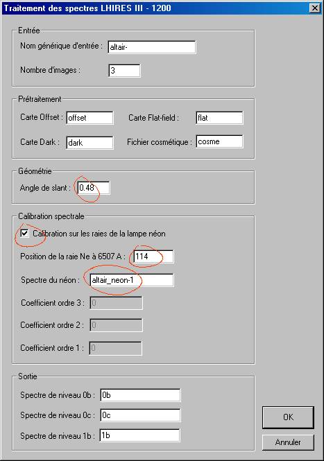
Enter the slant angle, the position of the line of neon at 6507 A and the file name of the neon file.  Click OK.

After a few seconds, SPiris will produce on  your hard drive a 2-D 0b level spectrum, a 0c level graph and a wavelength calibrated leve1b spectrum (sampled at 0,344 / pixel).

For spectral calibration, SPiris calculates a best fit third order polynomial to the position of the neon lines.  The RMS error is very small.  The parameters of the polynomial are returned in the output window (a3, a2, a1).  They can be used to calibrate other spectra in the observation session.

The Altair level 0b spectrum:

The 0c level spectrum in graphical form (using the command l_plot):

The level1b product (note that the wavelength calibration has been done here):

 4.2. Processing the spectrum of the star HD173292

With the star HD173292 we are dealing with a star much fainter than Altair.  It has a magnitude of V = 8.6, which is close to the faintest magnitude reasonably achievable with the LHIRES III spectrograph equipped with the 1200 lines / mm grating.  This object is a potential target of the Corot satellite.

Click here to download the raw images.

 We have 10 raw images each of 300 seconds.

do:

 >number  173292 -

Select the spectrum:

Then we open the treatment dialog box

 Here, the  0c level spectrum:

 The Halpha activity is easily seen in this rather extreme target after a cumulative exposure of 50 minutes.

 <home>     <next>    Page 1 / 6