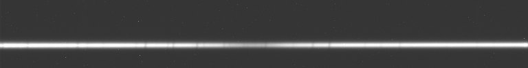
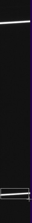
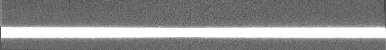
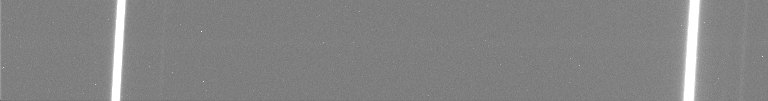
The raw 2D spectrum image, altair-1.pic. The, very large halpha line is visible in the centre. The thin lines are produced by atmospheric water vapour.
We have 3 spectra of the star Altair, each of 120 seconds exposure, taken successively. They have been saved under the names altair-1, altair-2, altair-3. The generic name of the series is "altair-”.
Here, we will break down the overall processing stated in Section 3 of this tutotrial.
Remember the method to find the number of images in a sequence:
>number altair-
To see the settings for the acquisition of the currently displayed image (exposure time, date of observation, etc ....) use
>info
This is the first spectrum of the sequence:
The raw 2D spectrum image, altair-1.pic. The, very large halpha line is visible in the centre. The thin lines are produced by atmospheric water vapour.
Note the format of the image. The CCD acquisition was windowed (using Pisco software, but most CCD acquisition software can do the same ). Normally a KAF-0400 series CCD has 768 x 512 pixels. Here we only keep an image 768 x 100 pixels. Those parts of the image rejected contain nothing of interest for spectrography, and they unnecessarily clutter the hard disk. In spectrographics, you can lose the habit to acquire the image as large as possible. Conversely, you should not crop the image extremely close to the transverse dispersion axis. The regions on both sides of the spectrum are very important to evaluate the background (see below). Finally, when choosing a window in the CCD image, we must stick to it, because you can then build a library of very useful and time-saving image masters.
During the adjustment of the spectrograph, more specifically, during the assembly of the CCD camera on the instrument, time should be taken to ensure that the axis of dispersion is exactly horizontal. The residual error here is less than 0.1°. You must try to level the axis of the spectrum to 0.2 or 0.3 ° degree at most. This can be done with a little practice (you must proceed through iterations).
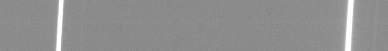
It should be noted that the Altair spectrum is not very well centred along the vertical axis. This is not dramatic, but we could do better ... The idea is to divide the sky evenly on both sides of the spectrum. We will see the importance of this later.
How can we measure the angle of the axis of dispersion of a spectrum relative to the sensor rows? SPiris / Iris has a small practical tool for this, the command l_ori.
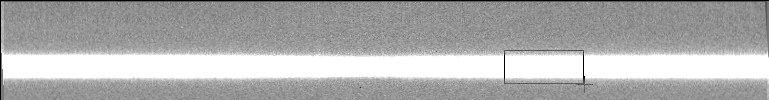
With the mouse pointer, draw a very elongated rectangle on the spectrum, as shown in the figure below:
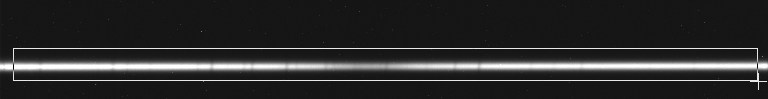
Spectrum Rectangle Selection (drag by pressing the right mouse button).
Avoid the extreme edges of the spectrum, but ensure that the length of the rectangle would encompass a large portion of the spectrum. Only worry about the right and left selection limits. The height of the rectangle does not matter. SPiris will use the ends of the spectrum so defined to calculate the angle of dispersion compared to the horizontal axis of the image. After drawing the rectangle, run the command l_ori (no parameters):
>l_ori
The result is returned in the output window. You will find approximately -0.062 °.
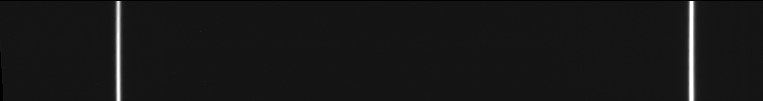
Associated with the three altair spectra is a spectrum of the LHIRES III internal spectral calibration lamp. It is the image altair_neon-1. Load it into memory:
>load altair_neon-1
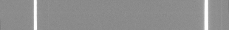
Neon spectrum around Halpha with a spectral sampling of 0115 A / pixel.
Two emission lines are visible at wavelengths of 6532,882 and 6598,953 A.
A high-contrast visualization of the spectrum shows other much weaker lines, not necessarily related to neon (presence of impurities?):
Viewing high contrast view of the neon spectrum.
At a height of 100 pixels the spectral lines should be vertical. Instead, they clearly appear slanted. We should not worry about this, this is normal with the LHIRES III. It is an optical distortion inherent in the optical design of the spectrograph. Do not try to make these lines vertical by rotating the camera. We saw that the proper orientation of the camera is so that the axis of dispersion is as horizontal as possible. This is the more important condition.
The angle of the lines from the vertical is of the order of 3 °.
It should be noted that the spectral lines of the stars are also suffering from the same slant. It is, however, less noticeable because the stellar spectra are narrow.
At this stage, it is very useful to know with a good accuracy the angle of inclination of the lines, say to 0.1 °. The l_ori command can help us. However, it can only accurately measure lines that deviate slightly from the horizontal. To use l_ori on the neon lines, the trick is to rotate the spectrum temporarily through 90° using:
>mirrorxy
Thus
Rotating the neon spectrum and measuring the slant of an emission line.
The average results for the two neon lines is 3.5°. One should remember this value. It is characteristic of your spectrograph and the position of your window in the CCD image. This parameter will vary only slightly from one night to another if you do not disassemble the instrument.
It is easy to check the exact angle by measuring lines with the slant command. Return the spectrum to horizontal (eg, with a second call of the mirrorxy command), then run the command:
> slant 50 -3.5
slant has two arguments:
- A coordinate along the vertical axis of the image with respect to which the points of the spectrum will be adjusted. The row at this coordinate is not changed, however, the rows above and below are corrected geometrically. The position of this coordinate (Y0) is not critical, but it is a very good habit is to always take the same value when processing spectra ( especially as geometric changes to a star spectrum affect the associated wavelength calibration). We choose the value Y0 = 50 because it is the centre of the image along the vertical axis (remember that the picture here has a height of 100 pixels). The value is also easy to remember.
- Adjust the angle of the lines, using the value which we calculated earlier (be careful with the sign).
Here is the result, the lines are now perfectly vertical:
Neon spectrum after application of the slant command.
It must be understood that the command slant does not rotate the image. The correction of the lines is obtained by dragging each row of the image sideways by the appropriate value. The fact there is no rotation is important to keep the dispersion axis horizontal (or at least as it was before using the slant command).
We can proceed with preprocessing the sequence "-altair”. This preprocessing is to subtract the offset , and dark and divide the result by the flat-field. These operations will be carried out automatically on all images in the sequence.
Load the first image of the series:
> load altair-1
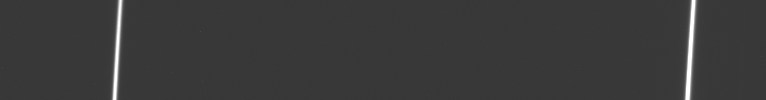
With the mouse pointer, select a fairly large rectangular area outside the spectrum:
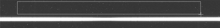
Selection of the area for calculating the optimal dark.
The pixels in this area will be used to assess the best factor to be applied to the thermal image (dark) to minimize noise in the preprocessed images.
Run the command Pretreatment of 2D spectra (basic) ... from the Spectro menu. Fill in the dialog box in the following manner:
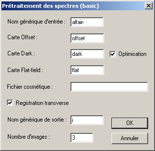
Pretreatment dialogue
Note: if you run the command number beforehand, some fields in this dialog box will be pre-filled.
Please check Optimization and transverse Registration.
The first option tells the program to automatically optimize the thermal signal within the area defined by the mouse just before opening the dialog box. This operation is especially needed here because we are going to process images with120 seconds exposure each, using a dark with an exposure time of 300 seconds. If you de-select the optimization option, the software performs a simple subtraction of the current image and dark.
The second option tells the program to align the spectra in the vertical direction (spectra index 2, 3, ... are aligned relative to the first spectrum in the sequence).
The offset dark and flat-field Fields are pre-filled. That's why, for convenience, the master images calculated previously were called offset dark and flat.
You must specify the generic name of the series of preprocessed spectra (the results of this calculation). In this example we will use the name "i", which means that we are going to produce in the working directory images i1, i2, and i3. Finally, we must provide the number of images in the sequence, here it is 3.
When you click OK the preprocessing begins.
The result is a sequence of three images i1, i2, I3 pretreated and aligned vertically relative to the first image in the series. In addition, SPiris adds these three images and displays the result. It is also in memory and you can save it to disk, for example by:
>save result
A variation on this preprocessing procedure is to include the automatic correction of cosmetic defects. Here we will remove most of the hot pixels using the file come.lst created when calculating the dark image. Just enter the name of the file containing the list of defects in the image in the cosmetics field (as always in Iris / SPIris, without the filename extension). We will therefore have:

Preprocessing including cosmetic correction.
Recall that the hot pixels are eliminated by interpollating from neighbouring pixels. The use of a "cosmetic" file identifying dozens of the most intense hot pixels is generally recommended.
The addition of the 3 pretreated spectra produces a level 0a product (see here the definitions of the levels of spectra).

Level 0a 2D spectrum of the star Altair.
To obtain a spectrum 0b level, it must be corrected geometrically and the sky background removed
Let us first consider the geometric corrections. In a spectra acquired with a LHIRES III and a 1200 l / mm or 2400 l / mm grating, there are only two types of geometric correction needed: (1) a "tilt" correction and (2) a "slant "correction.
The tilt angle is the lack of parallelism between the axis of spectrum dispersion and the rows of the sensor. We saw earlier that the command l_ori will find that angle. But the pretreatment command calculates it and displays the result in the output window. At the end of preprocessing, consult the output window. You will find something like:
Orientation: -0,057
The value -0.057 is the error in the parallelism of the dispersion axis in degrees.
Correct the image in memory (sum of the spectra of Altair 3) using the tilt command:
>tilt 380 -0,057
This command has two arguments. The first parameter is the pivotal position of the geometric transformation along the horizontal axis. It is a sort of neutral point: all other points of the spectrum are moved relative to it . The value has no critical impact on the outcome but it is best to choose a point close to the centre of the image. The image is 768 pixels wide, we have chosen the value 380. The most important thing is to always use the same value, especially if we geometrically transform the star spectrum and the neon spectrum that goes with it: the two should be corrected in the same way (see below).
You can also perform the tilt transformation from a dialog box. Open the Spectro menu and select Tilt of a 2D spectrum ...
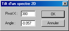
Tilt correction (tilting of the spectrum).
Note: correcting the tilt of the spectra apparently does not appear in the processing tools described in sections 3 and 4. This processing is in fact done, but it is hidden to the user; SPiris finds the angle of tilt for you.
The second correction to be made is the slant geometric correction (rotation of the spectral lines). After the latter, the spectral lines will be vertical. We can use the value found for the neon spectrum (it is almost a constant of the instrument. flexing of the spectrograph has little effect on the value of the slant angle):
>slant 50 -3.5
It is possible to make this correction from a dialog box. Open Slant of a 2D spectrum ... from the menu Spectro:
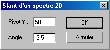
Slant correction (tilting of the spectral lines).
Both geometric corrections must be applied sequentially (it is recommended to correct the tilt first, then the slant) .. You can save the intermediate result if you are afraid of making a wrong move:
>save tmp
Altair spectrum after the geometric corrections.
It is instructive to examine the geometrically corrected image at high contrast, as is shown above. We note the presence of very faint neon lines. This is a problem peculiar to the CCD detector used. Here we see traces of the previous neon image, which fades slowly! It may be noted that these lines appear vertical, which was the purpose of geometric transformation. It is precisely because we have corrected the geometry of the 2D spectrum that we can easily elliminate these unwanted neon lines. Careful examination of the above image also shows that the brightness of each side of the spectrum is not zero (There is about 100 counts difference in the example - to view, move the mouse pointer and note the reading at the bottom of the image). The background is not strictly flat due to a slight light leak in the spectrograph (we must think about how to seal the instrument, if as is the case here, the ambient light pollution is high).
The next step is to subtract the sky background, we interpollate using both sides of the spectrum (hence the requirement to have the spectrum centered in the vertical, which is not really the case here). Although the operation is simple in principle, it is not very easy to achieve in an automated fashion. It takes a little care, and it must be remembered that it sets the zero level in our spectrum. The photometric quality of the final spectral profile depends heavily on the proper removal of the sky.
Load the geometrically corrected image (forslant and tilt). From the command line, run l_sky2 (without arguments):
>l_sky2
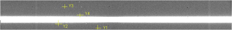
Apparently, nothing happens! But if you hold the mouse pointer on the picture, you will see that it has changed its shape. The arrow has turned into a cross. The software prompts you to click 4 times in the image to define the vertical coordinates y1, y2, y3 and y4. Choose positions such as indicated in the following figure:
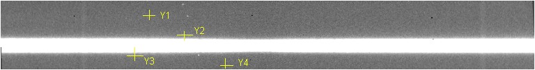
Interactive pointing to locate the sky.
As soon as the fourth point has been defined, SPiris calculates the background median value for each column in the image between the lines (Y1-Y2), and then between the lines (Y3, Y4). The average of these two values is then subtracted from the column in the image.
When chosing the points, only the vertical position (Y axis) matters. You can click anywhere you like along the horizontal axis.
It is important not to click too close to the spectrum of the star in order not to include any of the spectrum in the calculation of the sky. However it should not be too far away from the spectrum because the sky may be affected by slow variations in the background. To see the limits of the spectrum, we do not hesitate to "saturate" the view, as seen in the previous image.
One can imagine the importance of trying to centralise the spectrum. In the example suggested, the calculation of the sky is less accurate at the bottom compared with the top, due to the uneven number of pixels available to conduct the evaluation. If the accuracy of the telescope tracking does not easily position the spectrum at a sufficiently precise location on the entrance slit, you must expand the height of the images (from 100 to 150 pixels high, for example). The goal is to have reasonable size areas on both sides of the spectrum to evaluate the sky background (20 pixels wide at least).
The order of defining the four points is not critical. For example, you could have done:
Another order of valid points.
The only precaution to be taken is that couples (Y1-Y2) and (Y3, Y4) are identified on each side of the spectrum.
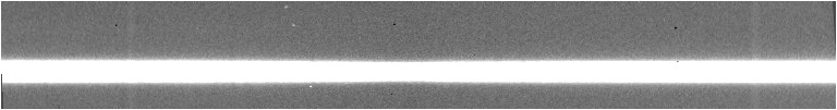
Here is the result of the removal of the sky:
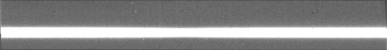
The 2D spectrum after the removal of the sky.
It may be noted that the neon parasites have disappeared. In addition, by moving the mouse pointer over the sky you will see that it has a zero value on average.
We have produced a level 0b spectrum: the dispersion axis is horizontal, spectral lines are vertical, the background level has been subtracted. You can save it to disk, for example:
>save taltair_1
(The "t" in front of the name of the star means it is a processed spectrum, and we use the "_" as a separator rather than "-" to better distinguish the processed image from the raw images - each person has their own file naming logic, but the most important thing is to stick to it).
Rather than run l_sky2 from the command line, you could have used the command subtraction of the sky from a 2D spectrum ... from the Spectro menu:
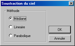
Subtraction of the background.
There are three interpolation options. We chose to calculate the median of the sky in the two areas on either side of the spectrum. This choice is correct here because the background is sufficiently homogeneous. If the background had a significant gradient along the vertical axis, it would be better to opt for a linear adjustment: the software then calculates a linear equation for each column and it is this model that is used to subtract the background . The adjustment equations are calculated by the least square method using parts of the image between (Y1-Y2) and (Y3-Y3). The equivalent command from the console is l_sky3. In the case of a difficult very irregular background, you can ask the adjustment to be made using a parabola (second order equation). The equivalent command is l_sky4.
Examination of the processed spectrum shows some bright spots and some black spots. They are either cosmic ray impacts or parasitic light affecting the images during the exposures. These artifacts can be troublesome if they occur on the spectrum, especially if the subject is weak. cosmic rays events are relatively frequent. Their probablity is far from zero. A strong cosmic impact in the sky area can make it difficult to properly assess the level of the background.
Statistical Methods applied to stacks of image sequences are very valuable to elliminate this type of defect in the 2D spectrum image. The median composite of a series of images, for example, is very efficient at rejecting points which have an abnormal intensity. There are other methods, almost as robust, which also retain the best signal to noise ratio. The technique of sigma-clipping it is probably the best known and one of the most effective. There are many other algortithms. SPiris (Iris) offers a variety of methods to reject outliers. Open the dialog box Add a sequence in the Processing menu .... Enter the generic name of the pretreated spectra adding (here "i") and the number of images in the sequence. Select Weighting adaptive and limit yourself to one or two iterations of the algorithm (that is sufficient in most cases). Click OK:
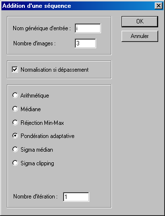
Optimal combination of images.
Adaptive weighting is a simple and effective method (a minimum of images are required). It is very commonly used to combine low-intensity LHIRES spectra (it is this method which was used in section 3 and 4). However, for these statistical methods to work properly it is necessary to meet two conditions:
-- Have a relatively high number of distinct spectra. In the example, 3 spectra is the bare minimum and 5 spectra is a reasonable minimum. If you have a dozen or more spectra, it's even better.
- The pixel intensities between the spectra must be relatively homogeneous or there is a risk of having all the information in a particular spectrum incorrectly identified as bad and rejected if it is significantly different from the others. The use of the command l_norm before stacking is then recommended to normalize the intensity of a sequence of spectra (you must select the spectrum in the first frame in the sequence to start with).
In difficult cases, cosmetic correction to the spectrum is possible using commands such as max and min.
Once the optimal stack has been produced, you just have to make the geometric corrections and subtract the sky background:
> slant 50 -3.5
> tilt 380 -0,057
> l_sky2
> save taltair_1
The final level 0b spectrum. Note that the cosmic impacts have disappeared, as well as the black pixels.
The next step is the extraction of the 1D profile spectrum from the level 0b 2D image. It uses the command l_opt.
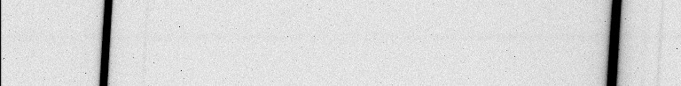
The use of l_opt is simple. View the 2D spectrum with a high contrast to see the limits. Using the mouse, define a rectangle that encompasses the spectrum along the vertical axis. The length of the rectangle does not matter. For example:
The binning operation.
Then run the command l_opt (no parameters):
>l_opt
The program calculates a 1D profile by adding the pixels in the 2D spectrum, column by column. The calculation uses pixels located between the upper and lower limits of the rectangle defined with the mouse. This calculation minimizes noise giving less importance to portions of the images that have received little starlight. The result appears on the screen:
![]()
The spectre 1D level 0c.
For easy viewing and manipulation SPiris displays the same row 20 times, but this is a 1D spectrum.
The profile can be viewed as simple graph using the command l_plot (the software displays the intensity of the first row at the bottom of the image in memory in the form of a graph):
>l_plot
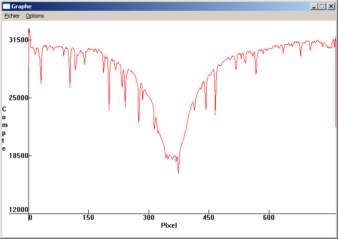
Spectral profile of the star Altair.
The spectrum is saved to disk in the form of a two column ASCII file (the first column contains the pixel number, the second column contains the intensity of the digital spectrum), you generate a product known as Level 1a. To save this ASCII file, use the File menu of the plot window
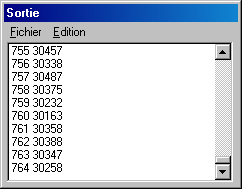
A product level 1a.
At this stage, the 2D image processing has been completed. The remaining operations are essentially spectral calibration and correction for the instrument response. They are done in specialized software, such VisualSpec. You can export your level spectrum 0c for example:
>save taltair_2
Normally you must also export the neon spectrum associated with the star spectrum if you want to perform spectral calibration using third party software.
Here is the spectrum altair_neon-1:
Raw spectrum.
The spectrum after subtraction of dark and offset:
Level 0a Spectrum.
The spectrum after the correction of geometric distortions:
>slant 50 -3.5
>tilt 380 -0,057
Spectrum level 0b.
The 1D spectrum with thirty rows binned around the position of the star spectrum:
> l_add 15 45
![]()
Spectrum level 0c.
The profile:
> l_plot
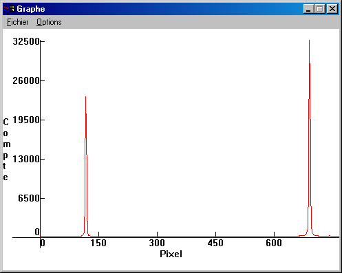
Profile of the spectral calibration lamp.
To make your own tests, you can:
-- download image taltair_1 (level 0b)
-- download image taltair_2 (level 0c)
<previous> <summary> <next > Page 3 / 6