SPECTROPHOTOMETRY
Practical examples using ISIS

Christian Buil


http://www.astrosurf.com/aras/


Cliquer ici pour une version en Français de cette page


SUMMARY

PART 1 : HOW TO EXPRESS SPECTRA IN ERNERGY UNIT
    - Method 1 : from 4 spectra
    - Method 2 : from 2 spectra

PART 2 : HOW TO EXTRACT MAGNITUDES FROM FLUX SPECTRA

PART 3 : HOW TO ATTACH DATA TO A PHOTOMETRIC SYSTEM

PART 4 : THE "INSTANT" MEASURE OF ATMOSPHERIC TRANSMISSION

PART 5 : HOW TO PREDICT THE PRODUCED SIGNAL BY A GIVEN STAR

In the part 1 we will consider two methods to convert spectra in units of relative intensity into ones expressed in physical units. The methods described are accurate spectrophotometric techniques that can for some studies, greatly enhance the value of the spectra.

Method 1 requires four spectra: narrow slit spectra of the target and a reference star in the sky nearby, and wide slit spectra of the target and reference.

Method 2 requires only two spectra: spectra of the target star and reference stars.

The second method is clearly the easiest and this is probably the "official" technique used at most observatories. It is less accurate than the first method, as the relative transmission of the slit between the measurements of the target and reference stars (with reference to the seeing quality, accuracy of the telescope guiding and the parallactic angle) may not be the same. To limit errors, I suggest using method 2 with a wide slit for applications that require high photometric accuracy.

Note that only method 2 can be used with fibre fed spectrographs.

Other methods are possible. See in particular this procedure (F. Teysseir) that mixes both traditional photometric imaging (with a band-pass filter) and spectrography, but less direct than the techniques presented here, which uses only spectral data and only one instrument.

Part 2 shows how to use the spectra expressed in energy units to extract the BRV magnitudes

Part 3 shows in a practical example how to establish the equations for attach your data to a photometric system and thus produce precise magnitude measures.

Part 4 is an exploitation of instrumental sensitivity evaluation for evaluate quickly the Earth atmospheric transmission.

Finally, part 5 is an exploitation of all that is said above to calculate the radiometric efficiency of observation system.
 

PART 1 : HOW TO EXPRESS SPECTRA IN ENERGY UNIT

METHOD 1 : from 4 spectra

STEP 1

I begin by describing the most complex method - a mix of high and low resolution spectroscopy... (the complexity is relative, there is nothing
really complicated in all that follows, just practice for perceiving it!)

First, load in memory software and display a  reference spectrum. Here the spectrum of the star HD196544, magnitude V = 5.428 , taken from the MILES database (this database is integrated into ISIS software). The spectrum is expressed in relative intensity (normalized to unity around 6700 A).

Save the profile as a FITS file. For example, the name: REF_HD196544.FIT


STEP 2

This reference profile is expressed in relative intensity (arbitrary units). Our goal is to convert it to a profile expressed in physical units. Here we choose ergs/cm2/s/A (energy flux).

This is possible because the V magnitude of the star is known (it is given in the catalog). Open the "Tools" tab, then the "process spectra 3" tab and complete the boxes as indicated in the screen shot on the right.

ISIS uses the following formula to perform the flux conversion :


STEP 3

The intensities in the REF_HD196544_FLUX.FIT file are now in physical units. View this spectrum in ISIS.

Note: ISIS 5.3.0 and above includes some of the CALSPEC database standard stars ( http://www.stsci.edu/hst/observatory/cdbs/calspec.html ) in which the spectra are measured experimentally and expressed directly in ergs/cm2/s/A. They are, however, relatively faint objects. If you work with bright targets, you can create your own spectrophotometric pseudo - standards by following steps 1 and 2.


STEP 4

Select a reference wavelength. Generally any wavelength can be chosen (4750, 5500 A, ...), but here a wavelength corresponding to a fairly flat region in the continuum of the target star spectrum has been selected (this is a spectrum of nova Delfini 2013 measured August 29.8 2013).

The selected reference wavelength is l o = 6100 A. T he flux of the MILES reference star at this wavelength, expressed in physical units is:

Fo = 1.81 x 10 -11 erg/cm2/s/A

(This is the flux outside the atmosphere).


STEP 5

The reduction of the target object spectrum is quite standard. This spectrum is observed with a narrow slit (here 23 microns wide). The result is expressed as relative intensity. This spectrum is designated by the letter 'a' . The instrumental setup used is an Alpy 600 spectrograph (R=600) on a Celestron 11 telescope (D=0.28 m). The science camera is the Atik460EX model.

On the right, is the reduced spectrum of nova Delphini 2013 in relative intensity (the region from 6650 A to 6680 A has been selected for normalization to 1, but you can make a different choice).

The relative intensity found at the reference wavelength (6100 A) in this example is:

Fa = 0.827

Note: The above spectrum was calculated by taking into account the attenuation due to the instrument and the atmosphere. The easiest way to estimate these parameters is to observe a star angularly close to the target, which alleviates the problems of atmospheric refraction and reduces the differential absorption. In the case of spectrum of nova Delfini 2013 'a' , it was reduced using a spectrum of the A2V type star HD196544 observed under the same conditions (23 microns slit) and located a small angular distance away.


STEP 6

The entrance slit attenuates some of the stellar flux. This attenuation is not constant over time. It is related to turbulence in the atmosphere, guiding errors, atmospheric chromatism , telescope chromatism...

To measure all the stellar flux independent of the slit effect, it is necessary to widen it. In the example on the right, I recorded a spectrum with an Alpy 600 spectrograph by temporarily positioning the star in the wide part of a special "photometric" slit. A convenient and powerful accessory here.

With a Lhires III or LISA spectrograph for example, you can simply remove the slit. The guider will not work, but this is not very critical if the objects are bright (short exposures - no guiding). The spectra are also a bit unfocused, but it is not a problem : the flux is diluted spatially and spectrally, but it is correctly measured. It is quite possible to swap over slits: if you have the possibility to use a wide slit while acquiring spectra, then it is worthwhile doing so .

The spectra of of both the target and reference stars should be measured using the same method.


STEP 7

Process the "photometric" spectra (obtained with a wide slit) as simply as possible.

First, enter zero values for the normalization zone ("Settings" tab). Also (very important), do not select the Weighted additionnal mode of individual spectra).

Choose a very wide binning zone to be sure to include all the stellar flux in the calculation of the spectral profile.

For processing , you do not even need to specify FLAT or instrumental response files.


STEP 8

Here the resulting "photometric" spectrum of the reference star.

The intensity is expressed in digital counts because we set the values in the normalising zone to zero .

We refer to this spectrum with the letter 'b' .

Measuring the signal at the reference wavelength we find:

Fb = 27020 ADU

The exposure time Tb is noted. Here Tb = 180 seconds .


STEP 9

The spectrum of the target object, the nova, is recorded and reduced in exactly the same way using a photometric slit (or with the slit removed) . We denote this spectrum by the letter 'c' .

The signal is measured at the reference wavelength

Fc = 7682 ADU

The exposure time is noted Tc. Here Tc = 150 seconds .


STEP 10

The coefficient C, which is the conversion factor between the relative intensity in the spectrum 'a' and the flux outside the atmosphere is calculated:

C = (Fo Fc Tb) / (Fa Fb Tc)

In the example:

C = (1.81 x 10-11 x 7682 x 180) / (0.827 x 27020 x 150)
= 7.47 x 10⁻¹²

We multiply the spectrum 'a' (measured using a narrow slit) by this value (see screen shot on the right).

Warning: it is assumed here that the target and reference star are observed at a similar air mass and within a short time interval (depending on the photometric quality of the night).


STEP 11

Here is the result, the spectrum of nova Delphini 2013 calibrated in absolute flux (ergs/cm2/s/A), as if the object was measured outside the Earth's atmosphere. This spectrum is now calibrated, ready for advanced astrophysical analysis.


METHOD 2 : from 2 spectra


STEP 1

The observed spectral profile of the reference star (here HD196544 ).

This profile is calibrated in wavelength, but it is not corrected for instrumental response. It is expressed in total counts for the full exposure time, which is here 6 x 30 s = 180 seconds.

Remember (see Method 1) to tell ISIS not to normalize the spectrum. Under the "settings" tab, enter zero values for the normalisation zone wavelengths.

To remove the effects of the slit, this spectrum was obtained with the Alpy 600 spectrograph using the photometric slit (width 230 microns).

Note that method 2 can be used in exactly the same way, regardless of whether the slit is narrow or wide. The risk of using a narrow slit though is significantly lower accuracy in flux.

Tip: Measure the signal as a series of 10 to 20 raw spectra of the same object and analyze the spread of the values. Any potential problem can usually be seen at this stage. The standard deviation of the distribution observed gives an idea of the measurement error. This is a way of testing the quality of your procedure.


STEP 2

The same profile as before, but expressed in counts per second per pixel instead of counts per pixel.

To produce this, the intensity of the spectrum measured in step 1 is simply divided by the exposure time (180 seconds).

This spectrum is called 'a' in what follows.


STEP 3

The spectrum of our pseudo standard (HD196544) taken from the MILES database and expressed in units of flux (see Method 1) .

The resolution of this spectrum has been degraded to match the resolution of the 600 Alpy spectrum by convolution with a Gaussian function (by using the "Filter" function in ISIS with a coefficient of 7).

This spectrum is called 'b' in what follows.


STEP 4

The spectrum 'a' / spectrum 'b' ratio.

The result is the the sensitivity curve for the instrumental chain. This includes the complete instrument (grating, detector, ...) but also the atmospheric extinction for the air mass for this observation.

However, the slit has no effect in this case as the slit is very large relative to the seeing disc.


STEP 5

The observed spectral profile of nova Delhini 2013.

Here the actual profile has been divided by the exposure time, which is 150 seconds. The measured intensities are therefore expressed in
ADU/s/pixel.


STEP 6

The end result: the spectrum of the nova measured in units of flux.

It is simply obtained by dividing the observed spectrum (in ADU/s/pixel) by the sensitivity curve.


COMPARAISON OF METHODS 1 ET 2

Here, a comparison of spectra produced by following Method 1 and
Method 2. The results are very close!

Although method 2 is the easiest (fewer measurements are needed) and is surely the procedure used in most observatories , it requires some precautions to be taken and has some limitations.

Details worth considering are ...


On examining the red part of the spectrum, we see that Method 2 has eliminated the telluric lines. This is as expected, because the sensitivity curve calculated in step 4 of method 2 includes the effect of atmospheric transmission. When we then perform step 6, the profile is automatically reduced to what it would be observed from space.

As a result, an emission line at 7250 A appears clearly in the spectrum obtained from method 2, while it is embedded in an absorption band from water vapour in the spectrum calculated using Method 1.


Now consider the blue part of the spectrum.

Method 1 clearly produces a spectral profile where the lines are more intense (and narrow ). The reason is simple: in method 2 the spectrum is here measured using a wide slit, hence the spectral resolution is degraded, and we see the effect of this.

In Method 2, the details in the profile are dependent on seeing and guiding errors. So be cautious when interpreting the shape and the peak intensity of the lines. The equivalent width however is unchanged between the two profiles.

One potential solution is to implement method 2, but using a narrow slit. But be careful though as the photometric distortions can be large if we observe away from the zenith and at a large parallactic angle. See in particular this page:

http://www.astrosurf.com/buil/alpy600/photometric_slit.htm

and the effects produced in extreme situations !

http://www.astrosurf.com/buil/dispersion/atmo.htm

The problems from the slit are reduced if the reference and target stars are nearby in angle (which should be the rule). Nonetheless potential photometric errors due to errors in positioning the star on a narrow slit remain. The advantage of the wide slit is that these effects are almost completely removed - spectrophotometric quality can then be better than a tenth of a magnitude.


In the ultraviolet part of the spectrum, method 2 has a higher noise than method 1.

This is due to the uncertainty in the the calculation of the sensitivity curve (step 4). If the spectra 'a' and 'b' do not have a very similar detailed profile, artifacts (pseudo noise) that have nothing to do with the actual response curve are produced.


To overcome this latter problem (which is rather serious, because in some circumstances it can lead to distortions in the lines which may be misinterpreted), I strongly recommend calculating a carefully smoothed response curve (eg using the "Continuum" tool ISIS). When calculating this, I ask the software to eliminate the telluric lines and the major hydrogen lines (the use of a flat-field image is also recommended i.e. a tunsgten spectra - here for remove fringing from the detector) .

This version of the instrument sensitivity curve (or instrument response) does not erase the telluric lines in the final profile (unfortunately). However, the increase in noise is minimized. It is a matter of choice.


The spectrum of nova Delphini 2013 reduced using method 2 and a smoothed sensitivity curve.


PART 2 : HOW TO EXTRACT MAGNITUDES FROM FLUX SPECTRA


STEP 1

Load and display analysed spectrum expressed in physical photometric unit (in erg/cm2/s/A) – The method for translate the intensities of a spectrum into physical units is explained in part 1 of the actual page.

The spectrum on the right is that of a photometric standard. It comes from the well-known Landolt stars photometric sequence. Professional astronomers use very often these objects to reduce the photometric data. There is a wide range of stars, mostly located in Selected Area (SA), of any spectral type, with precise BVRI magnitudes in the Johnson-Cousins
photometric system. They are very good secondary photometric standard for you. Here the spectrum of star SA 112-275.

See here for a list and field maps of Landolt standards: http://james.as.arizona.edu/ ~ psmith / tableA.html

The spectrum on the right is made with an Alpy 600 spectrograph + a Celestron 11 telescope (D = 0.28 m). The exposure time is 5 x 240 seconds. We use the spectral profile of star HD204041 for compute the system spectral sensitivity i.e. instrumentale global responsivity + atmosphere transmission (the original profile is extracted from the MILES database). I chose this object because it is at the same air mass that SA 113-475.

To convert observed counts to ergs/cm2/s/A I used method 2 discussed in
part 1.


STEP 2

Download the profile of synthetic spectral BVR Bessel bands system (see below). These cover the photovisuel field.

In blue side, the shortest valid wavelength is 3750 A. It is estimated that below this limit, the spectra show too much noise for correct results.

In red, the wavelength limit is 7400 A in order to avoid problems of order recovering, typical of grating based spectrographs - see at right. In other words, the R band is truncated in the red part. We see the consequences later.

Filter files:

BESSEL_B.FIT
BESSEL_V.FIT
BESSEL_R.FIT


STEP 3

Multiply the analysed profile star (in energy flux) by the profile of a synthettic filter, for example in the right screen copy with the Bessel B filter.

To do this, open the "Arithmetic" tool, and calculate the product of the two spectra. The result result appear in the Profile display tab (the screenshot correspond to ISIS V5.3.1).


STEP 4

The result is the weighted star profile by the transmission curve of numerical filter.


STEP 5

The energy flux through the filter is summed (numerical integration). To do this, open the "FWHM" tool, then double click on the far left of the profile, and then double-click just right, as the screenshot above shows.


STEP 6

Important information returned is the integrated energy flux, as it appears in the screenshot to the right. It is calculated by taking into account the sampling of the analyzed spectrum.

Here, the integral value for the B band:

Fb = 2.184 x 10⁻¹⁰ erg/cm2/s


STEP 7

You can do the same with the V and R filters (load the analysed spectrum before of course).

Here the results found for the V and R bands:

Fv = 4.048 x 10⁻¹⁰ erg/cm2/s

Fr = 1.751 x 10⁻¹⁰ erg/cm2/s


STEP 8

It remains to calculate the B, V and R magnitudes associated with the flux values found.

First, the instrumental magnitudes are estimated using the Pogson formula:

Bo = -2.5 log (Fb)
Vo = -2.5 log (Fv)
Ro = -2.5 log (Fr)

For the example:

Bo = 24.152
Vo = 23.636
Ro = 23,068

The conversion between the instrumental magnitudes (Bo, Vo, Ro) and magnitudes expressed in the Johnson-Cousins system is directed by a simple linear equation set (warning, the parameters are specifics to the instrumentation used, here a C11 telescope and an Alpy 600 a spectrograph coupled to a model Atik460EX CCD camera):

B = Bo - 13.028 - 0.01 x (Bo - Vo)
V = Vo - 13.730
R = Ro - 13.753 - 0.10 x (Vo - Ro)

The numerical application:

B= 11.119
V = 9.906
R = 9.258

Remember, Landolt magnitudes are B = 11.115, V = 9.905 and R = 9.258. The agreement is close to the hundredth of magnitude, which is a very good photometry.

A question arises: how are evalued the terms in the tranfert equations between instrumental magnitudes and real magnitudes (attached to a photometric system) ? These parameters are associated to a particular instrument and therefore they should be evaluated by you at least once (as they are very stable, you will rarely have to go back, only to refine your model).

The answer to this important question is the subject of the next part 3.


PART 3 : HOW TO ATTACH DATA TO A PHOTOMETRIC SYSTEM

Traditionally, the relationship between instrumental magnitudes Bo, Vo, Ro and photometric magnitudes B, V, R is done through a simple system of linear equations:

B = Bo - Zb - ab x (Bo - Vo)
V = Vo - Zv - av x (Bo - Vo)
R = Ro - Zr - ar x (Vo - Ro)

with Zb, Zv and Zr, the zero points of the magnitude scale, respectively for bands B, V and R.

ab, av and ar, are colors terms, which are used to correct the effect of the difference between the effective spectral filters bandwidth  (and instrumental chain ) and the bandwidth used by Landolt when establishing its photometric catalog. It is estimated that the filter system used is consistent with the photometric system if values of coefficients ab, av and ar are less than 0.5. This condition can reduce errors when measuring peculiar spectra (Mira, nova, ...).

To evaluate the terms in the tranfert equations, I observe three stars of Landolt sequences (located in the equatorial zone) with the C11 + Alpy 600. Here the stars selected with catalog data:

Name

Magnitude B

Magnitude V

Magnitude R

SA 112 275

11.115

9,.905

9.258

SA 113 466

10.458

10.004

9.723

SA 113 475

11.364

10.306

9.736

The response curve of the system, or system sensitivity, is computed from the observation of  star HD204041, located at the same air mass as the Landolt stars :

The observed spectrum of the secondary standard HD204041. The exposure time is 6 x 40 seconds. The signal here, in numerical counts, is reduced to an equivalent one second exposure.

MILES spectrum of HD204041 converted in flux.


The ratio of the two previous spectra gives the sensitivity of the system (for the effective air mass). This is the conversion curves to apply to convert the observed counts per seconds (ADU/s) to erg/cm2/s/A.
See details in part 1 - method 2.

Here the spectrum of the three observed Landolt stars. The spectra are converted into flux unit through the sensitivity curve previously established:

In all three spectra, the integrated flux is calculated in the Bessel BVR bands, following the method presented in the first part of this page, as well as the instrumental magnitude. The following tables show the results of measurements. We recall in the tables the Landolt magnitude expected. Finally, we give the zero point computed by using the simplified following transfert formulas (I do not consider color terms for the moment):

B = Bo - Zb
V = Vo - Zv
R = Ro - Zr

SA 112-275

B

V

R

Measured flux (Fb, Fv, Fr) in erg/cm2/s

2.184 x 10⁻¹⁰

3.511 x 10⁻¹⁰

5.926 x 10⁻¹⁰

Instrumentale magnitude (Bo, Vo, Ro)

24.152

23.636

23.068

Catalog magnitude (B, V, R)

11.115

9.905

9.258

Zb, Zv, Zr

13.037

13.731

13.939


SA 113-466

B

V

R

Measured flux (Fb, Fv, Fr) in erg/cm2/s

4.048 x 10-10

3.205 x 10⁻¹⁰

3.983 x 10-10

Instrumental magnitude (Bo, Vo, Ro)

23.482

23.735

23.499

Catalog magnitude (B, V, R)

10.458

10.004

9.723

Zb, Zv, Zr

13.024

13.731

13.776


SA 113-475

B

V

R

Measured flux (Fb, Fv, Fr) in erg/cm2/s

1.751 x 10-10

2.434 x 10-10

3.841 x 10-10

Instrumental magnitude (Bo, Vo, Ro)

24.392

24.034

23.539

Catalog magnitude (B, V, R)

11.364

10.306

9.736

Zb, Zv, Zr

13.027

13.728

13.803

Despite the non-inclusion of the color terms color, zero magnitude point (per band) is remarkably constant for the observed stars. This validate the procedure and the use of a low cost spectrograph for high quality photometric measures. The adopted BVR synthetic filter set is very near origibal Johnson filter set. Dispersion of zero point is of the order of 1/100 in B and V. The result is less good for the R band because truncation of the filter at 7400 A.

By hand, we can find a color term which enhances the R band photometry (the color coefficient found is is only 0.1 in R band and 0.01 in the B band, that is to say almost nothing for B). Here the final adopted equations (by exploiting only three stars Landolt):

B = Bo - 13.028 - 0.01 x (Bo - Vo)
V = Vo - 13.730
R = Ro - 13.753 - 0.10 x (Vo - Ro)

With this system of equations, the residual errors:

SA 112-275

B

V

R

Measured magnitude

11.119

9.906

9.258

Catalog magnitude

11.115

9.905

9.258

Difference (measured - catalog)

+0.004

+0.001

+0.000


SA 113-466

B

V

R

Measured magnitude

10.457

10.005

9.722

Catalog magnitude

10.458

10.004

9.723

Difference (measured - catalog)

-0.001

+0.001

-0.001


SA 113-475

B

V

R

Measured magnitude

11.361

10.304

9.736

Catalog magnitude

11.364

10.306

9.736

Difference (mesured - catalog)

-0.003

-0.002

+0.000

The observed precision is significantly better than 0.01 magnitude (with the caution of low number star observed).

This analysis makes the link between spectroscopy and photometry. It shows for some applications the possibility to substitute traditional photometry by spectrophotometry. One can also note an important difference: classical photometry produced only three information elements in the photovisuel domain, whereas with a spectrometer, several hundred informations elements are simultaneously extracted from the signal.

To conclude this section, a method for checking the set of photometric equations (from instrumental to real magnitude). The ISIS software database actually contains all the elements to verify the above calculations. Based on the spectra of stars already flux calibrated and applying BRV digital filters, we can ensure that the magnitude values calculated are coherents with the literature values. Here an example.

In ISIS, from the "Profile" tab, open the "Database" tool. In the sub-base CALSPEC, choose the star BD +25 4655, and then click the "Disply" button:

The star BD +25 4655 is a fairly bright spectrophotometric standard, often used in terrestrial and space-based observatories for flux calibration of spectra acquired with instruments. This is a very hot star (Teff = 43000 K), low hydrogen and helium rich. The lines of neutral and ionized helium once dominate the spectrum. The hydrogen lines are discrete and continuum is relatively flat:

From the tool "Arithmetic", multiply the spectrum by the profile of Bessel B:

Then, calculate the integrated flux in B band filter with the "FWHM" tool. Here we find Fb = 1.076 x 10⁻⁹ erg/cm2/s. Translated into instrumental magnitude with the help of the Pogson formula Pogson, this flux corresponds to Bo = +22.420.

The same calculation using the R Bessel filter provides for the star BD +25 4655, Fv = 4.401 x 10⁻¹⁰ and Vo = +23.391.

The Bo-Vo index is here Bo-Vo = -0.971. By introducing these values in passage formulae we find for this star:

B = 9.40
V = 9.66

The SIMBAD values for the same object are:

B = 9.39
V = 9.68

The difference is only a few hundredths of magnitude. Our formulas are correct.

Still for verification (and exercise), you can physically observe the reference star and thus, control globally the accuracy of your work.

Below there is an observed spectrum of BD +25 4655 with a Celestron 11 and a Alpy 600 spectrograph. The signal to noise ratio is very high, which is the primary guarantor of good measure:


PART 4 :
THE "INSTANT" MEASURE OF ATMOSPHERIC TRANSMISSION

We show in this section how to evaluate quickly the atmospheric transmission at a given moment of the night. The procedure is expeditious, as it is limited to photometric observation mode and concern only two stars insequence at different air masses. The time interval between the two measurements can (and should) be short. Typically, in my situation, the whole procedure takes less than 10 minutes, including the the telescope pointing
.
If possible choose first a fairly low elevation above horizon, between 25 and 35°. The second star is selected near the zenith (but not mandatory).

In addition, the method described is quick, so it can be renewed regularly during the night to follow the variation of the extinction of the atmosphere if needed. The evaluation of the atmospheric transmission can still improve the accuracy of flux measurement (part 1) if the reference star and the star calibrate have slightly in different elevations above the horizon (see below).


STEP 1

The graph to the right shows the sensitivity curves (see Part 1,Method 2, Step 4) calculated from two stars located at different elevations. Remember that the sensitivity curve represent here the number of digital counts observed in the spectral profile (per sample) for a given flux "out of the atmosphere" of 1 erg/cm2/s/A.

The sensitivity curve therefore includes both the overall performance of
the instrument, but also atmospheric transmission. This is the reason of difference of the sensitivity curve for the two stars. I select:.

- HD198001 (present in the MILES catalog) observed the 11.8699/09/2013 at an angular height of 36.6°, which corresponds to an air mass
a1 = 1.671.

- HD196544 (MILES catalogs) observed the 11.8610/09/2013 at an angular height of 57.70°, and air mass a2 = 1.183.

Tip: To calculate the air mass of an object from these coordinates
equatorial and the date of observation, use the Mis / Heliocentric velocity tab tool. Remember to enter your geographic coordinates in Settings tab and provide the days in fractional values, example: 11.8699).


STEP 2

The calculation method to find the atmospheric transmission from spectrum of two stars is detailed here. It is ideally suited to our problem.

We begin by calculating the inverse of the difference in air masses:

1 / (a1 - a2) = 1 / (1.671 - 1.183) = 2.049

Load into memory the first sensitivity curve, calculated by using HD198001 (see right).


STEP 3

Open "Arithmetic" tool from the "Profile" tab.

Start by dividing the sensitivity curve in memory of the second (the file is called here _sensitivity_hd196544).

The ratio of the two curves of sensitivity is calculated when you click the "Calculate" button.

Meaning leave "Arithmetic" tool, elevate the result to power 2.049 (see previous step).

Exit the tool.


STEP 4

The right graph shows the result of operations. This is the zenith absolute atmospheric transmission of the observatory.

Note that the result is significantly noisy. This comes to much from the short exposure time during the observation these stars (only 2.3 seconds). This noise is not very critical here because the purpose of this curve is only to adjust the ISIS atmosphere transmission model.

The parameter to adjust is the AOD index (Aerosol Optical Depth), which reflects the dust level in the atmosphere at the time of observation.


STEP 5

A synthetic atmospheric transmission curve can be calculated from the "Atmosphere" tool, see right.

By trial and error we find the value of AOD that fits best observation. Note that the calculation is fast.


STEP 6

Here the comparison of measured transmission with AOD = 0.14 synthetic atmosphere transmission (use the "Compare" tool of "Profile" tab. The agreement is satisfactory.

Finally, a synthetic atmospheric transmission model is adopted with
AOD = 0.14.


STEP 7

The spectrum of HD196544 star is used to flux calibrate the nova
Delpini 2013 spectrum (see Part 1). The declination of the reference stae is 11°22', while the nova declinaison is 20°46'. The small differential air mass between the two stars is at origin of a small systematic error in the computed nova flux.

We will evaluate this error.

During the observations, the air mass traversed by the light of the nova a = 1.085 (67.19° elevation), while for the reference star it is 1,183 (57.70° elevation).

The corresponding transmissions are calculated with the following tool ISIS modeling.


STEP 8

Because the nova (target) is higher in the sky as the star of reference (ref), the brightness of the nova is overvalued. We must apply a correction term for a more accurate flux evaluation. This term value (function of wavelength) is given by the ratio:

Correction = Transmission atmosphere (reference) / Transmission atmosphere (target)

In this case, the error caused by the difference in air mass and target is 2% in the red (equivalent to 0.02 magnitude) and 6% in the blue (equivalent to 0.07 magnitude).


STEP 9

It remains to apply the correction.

Load the spectrum of the target flux spectrum and multiply it by the correction term profile.

In this way, a large part of the spectral bias induced by differential between the height of the reference stars and the target is eliminated.


PART 5 :
HOW TO PREDICT THE PRODUCED SIGNAL BY A GIVEN STAR

We describe here 
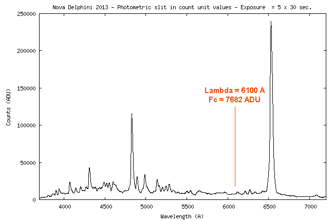
the workflow for predicting the measured number of digital counts in spectrum chosen point of the signal for a given star given.

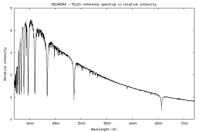
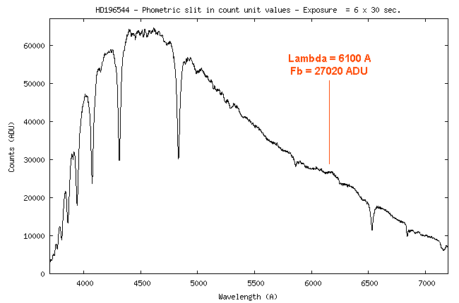
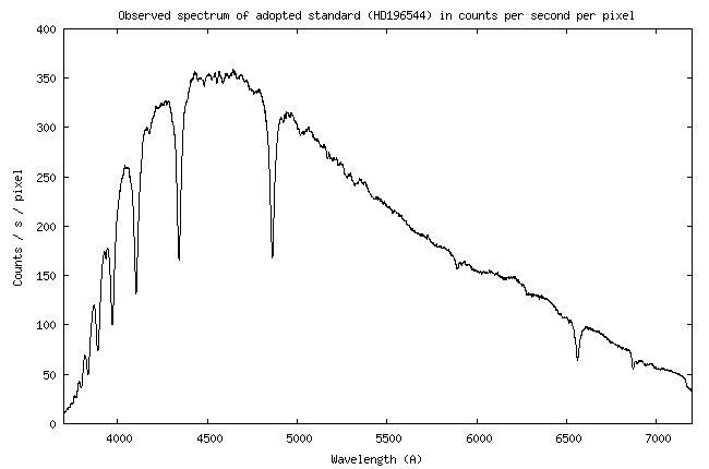
For this demonstration I will be using the instrumental 
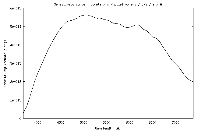
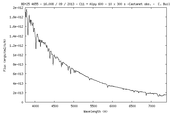
system sensitivity curve established during the observation of star HD196544, while it was at an elevation of 57.08 ° above the horizon (an air mass of 1.191). During the night of observation in question, the atmosphere was very pure. the AOD (Aerosol Optical Depth) was measured at 0.09 from the observation of two stars at different elevations (see section 4).

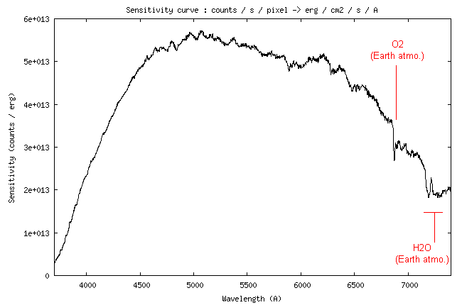
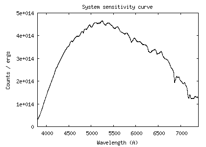
Here the sensitivity curve:

I remember that this curve is the link between the digital counts (the signal inADU = Analog Digital Unit) observed in a sample of the spectrum (after of course removing the offset signal, the thermal signal and the sky background) and a flux of 1 erg/cm2/s/A at the telescope entrance for the given wavelength (see Part 1, Method 2). The sensitivity is reduced to an exposure time of 1 second.

The telescope is a Celestron 11, the spectrograph is an Alpy 600 and the camera amodel Atik460EX operated binning 2x2. I arbitrarily select to perform the calculation at the wavelength of 5550 A. Of course, you can select any other point of the spectrum.

At the wavelength of 5550 A, the value of the instrumental sensitivity is 4.26 x 10¹⁴ (ADU)/(erg) - see the curve.

We will calculate the number of ADU that would be measured if the instrument was located outside the Earth's atmosphere. Atmospheric transmission is calculated by using "Miscellaneous" tab and "Atmosphere" tool for a star elevation of H = 57.08° and AOD = 0.09.

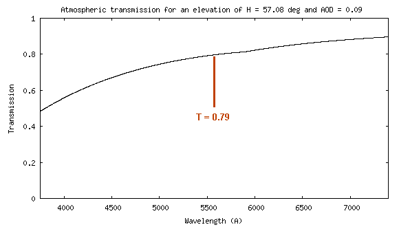
The observed signal outside the atmosphere would be: So = 4.26 x 10¹⁴ / 0.79 = 5.39 x 10¹⁴ (ADU)/(erg).

This is the value that we will try to find by calculation.

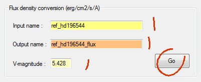
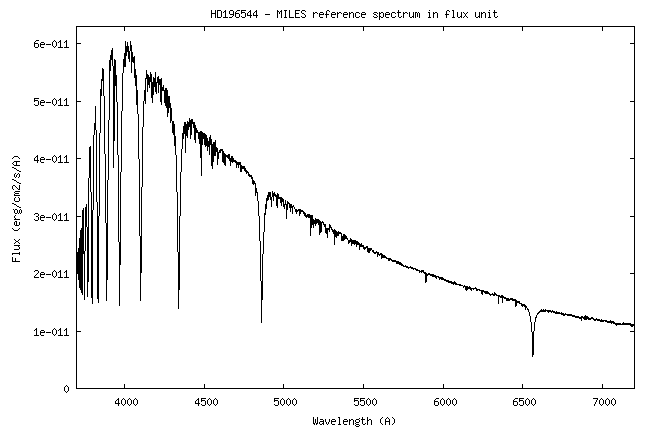
This means a star outside the atmosphere producing a flux Fo = 1 erg/cm2/s/A.

For convenience, this energy  flux is converted into a photons flux (photons/cm2/s/A).

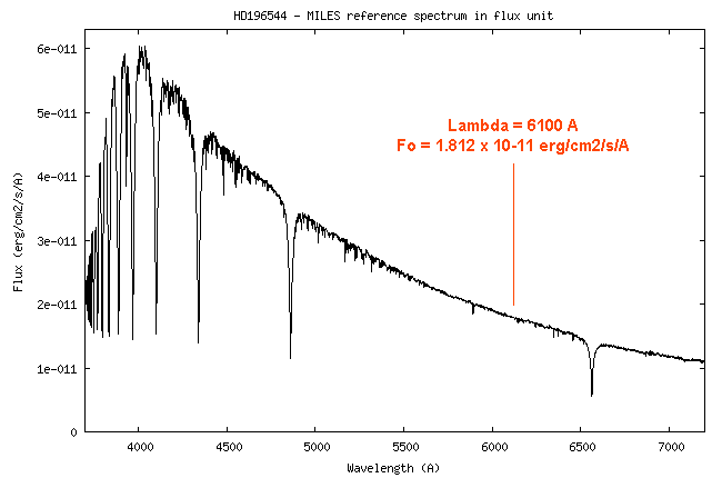
The conversion formula between the flux expressed in ergs and the flux expressed in photons is

No = (Fo x W) / (1.9861 x 10⁻⁸)

with the wavelength in Angstroms.

Doing the numerical application:

:No = (1 x 5550) / (1.9861 x 10⁻⁸) = 2.79 x 10¹¹ photons/cm2/s/A

This is exactly the number of photons received from our star in an area of 1 cm2, per second, per one angstroms bandwith above the Earth's atmosphere.

Our Celestron 11 has a diameter of D = 28 cm and a central obstruction of 0.357. Is easily to calculate the collecting surface with these parameters:

S = 537 cm2 (S = p  x 282 / 4 x (1 - 0.357) = 537 cm2).

The number of photons collected by the telescope pupil is: N1 = S x N = 537 x 2.79 x 1011 = 1.50 x 10¹⁴ photons/s/A.

Around the wavelength 5550 A, the Alpy 600 spectrum is sampled by the camera pixels with a pitch of 4.914 A/pixel (in bin 2x2 mode).

Tip: how to find this sample value? From the ISIS command line, run the following command (there are no parameters):

>DISPERSION

This function generates in the working directory a DISPERSION.LST file containing the value of the spectral dispersion as a function of wavelength (ISIS uses for this the dispersion equation you calculated previously for process the spectra). Here is an excerpt of this file:

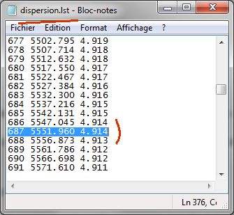
The first column is the pixel number along the axis of dispersion axis (as a detector coordinate), the second is the associated wavelength, the third is the reciprocal dispersion in A/pixel. We recover the value of 4.914 A/pixel announced.

In the spectral interval corresponding to a spectral sample, the number of incident photons every second is:

N2 = 4.914 x N1 =  4.914 x 1.50 x 1014 = 7.37 x 10¹⁴ photons/s

For an integration time t, counted in seconds, the number of photons will N3 = t x N2. Here, the reference time observation is t = 1 second, so

N3 = t x N2 = 7.37 x 10¹⁴ photons.

The optical transmission associated with the telescope and focal reducer is evaluated to 0.85. This value is the result of the product of the transmission of the entrance plate, the reflection coefficient of both mirrors (StarBrigth) and transmission of the focal reducer lenses.

The photon flux arriving at the entrance slit is N4 = 0.85 x N3 = 0.85 x 7.37 x 1014 = 6.26 x 10¹⁴ photons. For the moment we consider that the optical transmission of the spectrograph is 1 (ie, perfectly transparent to light). In making this hypothesis, the N4 photon flux reaches the detector.

Knowing the quantum efficiency of the detector at 5550 A, the optical signal is easily converted in photoelectrons per second. The approximate CCD quantum efficicency of Atik460EX camera (Sony ICX694EX) is given here. Value adopted is QE = 0.76 around 5550 A wavelength.

The number of photoelectrons for our incident flux density is N5 = QE x N4 = 0.76 x 6.26 x 1014 = 4.76 x 10¹⁴ electrons. In this same page, given with reference to above, we find that the electronic gain of Atik460EX camera is G = 0.260 electron/ADU. So, the expected signal (or calculated) in counts number is

Sc = N5 / G = 4.76 x 10¹⁴ / 0,.260 = 1.83 x 10¹⁵ (ADU)/(erg)

This result is compared to the signal actually observed, So = 5.39 x 10¹⁴ (ADU)/(erg) .

We explain the difference in the actual efficency of Alpy 600 spectrograph (its optical transmission), we have not seen before. This efficency is given by the ratio
Rs = So / Sc, so
Rs = 5.39 x 10¹⁴ / 1.83 x 1015 = 0.29

This transmission coefficient is an important feature of the instrument. Of course, the more the result is close to 1, the better is the spectrograph efficiency. I invite you to make this calculation and calculate for yourself the performance of your own instrument.

In the present situation, Rs is equal to the product of the transmission of both sides of the slit parallel plate, two objective lenses, the dispersive element (a grism) and the entrance window of CCD camera. The seeing does not impact here the result, because here the observation is made with a wide slit, much larger than the seeing disk (a 230 microns slit). If you work with a narrow slit, the performance  can drop be a factor 2 for example, because presence of seeing and guidance errors (function of slit width). These losses at the slit level are to be recognized in the calculation of Rs.

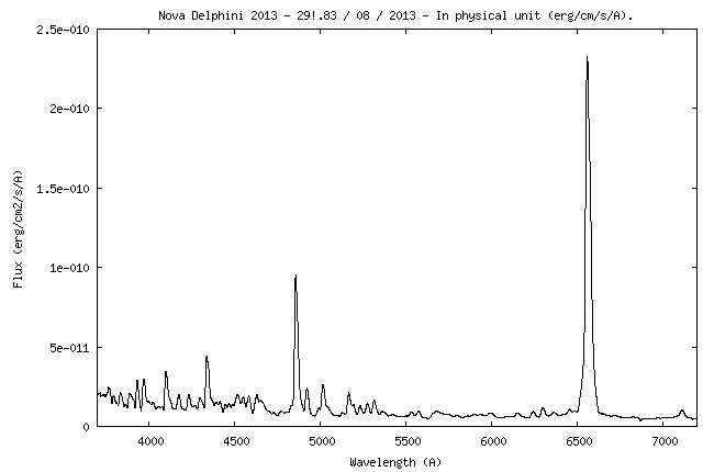
You now have all the elements to evaluate the expected signal produced in the spectrum for any star. Depending on the magnitude of the star, you calculate flux energy in ergs/cm2/s/A (for a wavelength of your choice). You multiply this result by the spectral sample bandwidth, by atmospheric transmission, by the surface of the telescope, by the optical transmission of the telescope and the optical transmission of the spectrograph (made a experimental estimate of this parameter in advance, as just explained). Then, convert the flux number of photons into electrons by using detector quantun efficiency. Finally, the ADU number is given by the camera electronic gain. Of course, if the exposure time is not equal to 1 second, you multiply the result by the exposure time in seconds.

Note: Be careful with the integration time with some cameras and/or acquisition software. Thus in the example, the consigned integration time when observing the star HD196544 was 2.30 seconds. But a simple test shows that this is not the true exposure time because the internal camera software or acquisition software generate a rounding error. It is easy to notice by making a 23 seconds exposure (23 = 10 x 2.3). The anomaly exists if the recorded signal is not precisely 10 times. Otherwise, you must correct the exposure time (reliable value is the long long exposure, because rounding potentiel error effect is greatly reduced). In our example, it turns out that the effective exposure time is not 2.30 seconds, but 2.49 seconds ! The error is about 8%, or 0,086 magnitude, which is not negligible when trying to perform accurate spectrophotometric measurements. To prevent this, I always try (if the exposure time is short) to observe the target star and the comparison star with the same integration time. This is the origin of the 2.30 
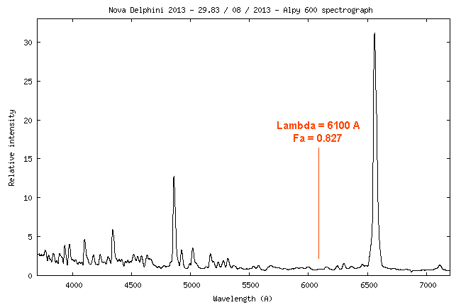
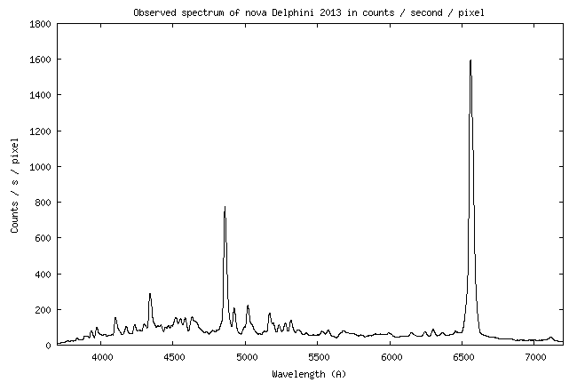
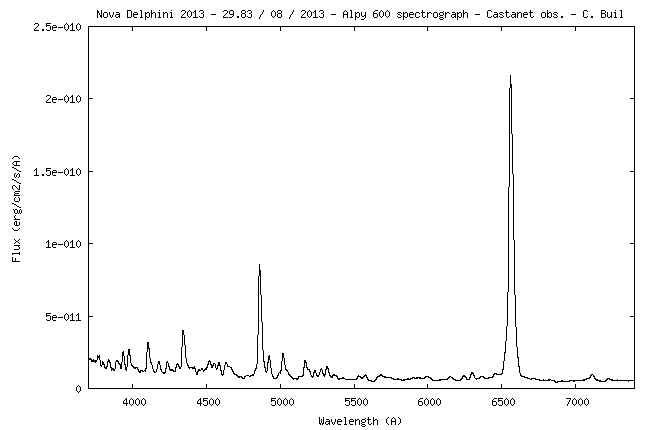
seconds exposure for HD196544, which may seem strange. In fact , this duration has been fixed during the observation of the nova Delphini 2013 (our target) will not saturate any part of the spectrum with the equipment described. So, I adopted the same exposure time for reference (HD196544 ) to avoid any problems (although in these conditions, the refrence spectrum is underexposed - to compensate I have accumulated a large number of images).


Back