
Page (3/3)
8. Improve color image
The image after preprocessing...:
One finds the dominant green tone (do not panic!), still accentuated by the light pollution which produces a significant and progressive gradient in the image top to downwards. We can see also the effect of the slight shift between each exposure: a nonrecovery zone appears on the edges. We will correct this last problem in priority.
If it is not already the case, first of all make a backup copy of the image, it is more careful:
SAVE T
IRIS proposes an interactive method to crop an image through a contextual menu. With the mouse drag the zone of the image which you want to preserve, then call the contextual menu (a right click of the mouse anywhere in the image). Finally run the Window command:
This method is efficient only if the part of the image to retain is smaller than the screen. For large images, coming from modern digital cameras it is necessary to note the coordinates of two points diametrically opposite which delimit the zone to be preserved, then to run the Window... command of the Geometry menu. Enter then the coordinates of the couple of points, then click OK :

A similar action can be obtained since the command line:
WINDOW 40 75 3050 2050
Tip: a technique to avoid noting the coordinates on a paper consists in displaying the window data output (last command in the list of the Analysis menu). Each time click in the image, the coordinates of the corresponding point appear in the output window:

A third method, more interactive, to crop a great image. Simply type the command WIN in the console. After the < Return > the mouse cursor takes the form of a cross. Made a first click in one of the corners image. Go in the opposite corner and made another click. It is all, the image is cropped automatically.
We now will give a neutral tone to the sky background, a natural gray aspect. For that the software will calculate a constant for each color layers which will be added or subtracted for equalize the sky background for the three layers (in fact the sky background is at zero level after equalization). The calculation is done a selected part of the image. With the mouse to delimit this zone (avoid nebulae!)
Then, simply enter the command BLACK in the console. Here the result:

For visualization use some things as:
VISU 900 -250
Note the negative value for the low threshold, which avoids having a ink black sky, for favorise the visualization of the weak details of the image.
The following step consists in multiplying each color layers by a constant so that a given star of the image appear rigorously white. Often one selects a star of the spectral type near of the Sun (type G2V). It is obviously passably arbitrary, but since a criterion should be found... It is IRIS which will calculate for you the good coefficients. The selected star is chosen by a small rectangle with the assistance of the mouse (use an unsatured star):
After, just after command WHITE2. This one carries out a Gaussian adjustment of star selected by the method of least square to find the intensity in each layer and the coefficient are applied (the coefficient values are returned by the program).
Note: we already use a similar command during the processing of the butterfly image, the command WHITE. This one calculates the multiplicative coefficients starting from the median value of a range of pixels selected with the mouse. WHITE2 on the other hand carries out a photometric analysis of stars so that this command is reserved only for deep-sky astronomical image.
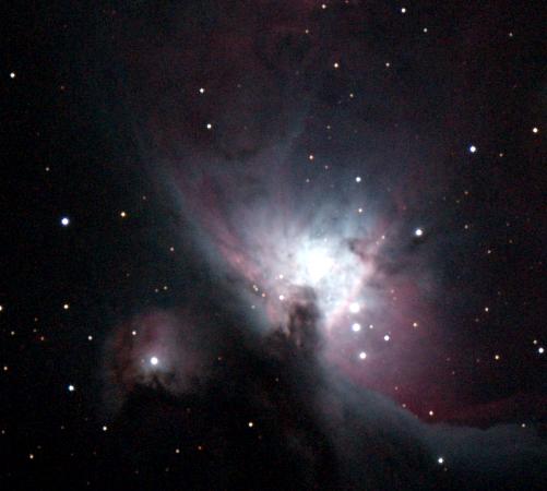
In this example, despite the efforts the nebula remains of bluish color whereas one would rather expect to see the red color of the line H-alpha line. The chromatic balance is now quite effective for stars, but the problem comes from the defect of sensitivity of the camera used in the far red, where the line H-alpha is. This completely unbalances the visual aspect of nebula, even if the stars are well represented. To find a traditional aspect for M42 it is necessary to manually by increasing the importance of the red to the detriment of the green and blue. One uses the White balance dialog box à View... menu:

You can visualizes better the great dynamics of the image by using tool DDP tool of the Visualization menu:

9. How to have a flat sky background?
The examination of our image reveals a nonuniform sky due to the difficult acquisition conditions: the day of full the Moon and a large level of city light pollution:
In this case you can adjust a synthetic sky which is then subtracted from the image to find a uniform bottom of sky. IRIS calculates the sky background by using the image to treat itself by defining a certain number of points distributed randomly in the image, but by carefully avoiding stars and nebulas. A polynomial surface of chosen degree by the user and passing as well as possible by the points is then calculated, then subtracted to the processed image. This operation is automatic: open the dialog box Background fit... from the Processing menu:

Sigma coefficient is a parameter of rejection to prevent that too many points are found in the diffuse nebulae or galaxies. A small value for this parameter makes it possible to prevent that nebulas are confused with the sky background, but while going too far in this direction the risk is to have enough points to have a precise adjustment. A polynomial order of 2 or 3 is generally sufficient (the max. value is 7). After the calculation, the points chosen by the program are shows in the form of small crosses. To see the processed image it is necessary to refresh the display, for example by readjusting the visualisation thresholds. Here the result in our example:

Note: you can also manually point pixels with the hand (with the mouse more precisely) by which IRIS will adjust polynomial function. This procedure only only work on monochromic images. For example suppose that you want to rectify the sky background of the red layer, here how to proceed:
SAVE_TR R G B (RGB
layer separation)
LOAD R
(loading the red layer)
POINTON (pass in
pointing mode for the cursor)
To carry out the pointings distributed well,
and avoid stars and nebulas
(you can realize 2000 pointings)
POLY 7 (compute
the polynom, in this example of the maximum possible degree 7)
SYNTHE (production of the
synthetic sky background)
SAVE TMP
(save
the artificial sky background)
LOAD R (re-load of the R
layer)
SUB TMP 0
(subtraction of artificial
sky, one
does not add a constant to the result)
SAVE
R2 (save
the result)
POINTOFF (leave the
pointing mode)
TR R2 G B (display of the new color
image)
10. How to modify the scale of the image?
To increase the size of a part of the image, select the zone in question with the mouse, then from the contextual menu (click right in the image) run the command Resample... command. Choose for example the Spline method for the interpolation which gives a very soft result, then the scale factor (higher than 1 for zoom-in and lower than 1 for zoom-out).


When it is a question the scale the total size of an astronomical image, prefer the command Resample... from the menu Geometry and alternatively the Binning... command in the same menu. The binning is a well-known operation of the users of CCD cameras. It consists in adding the intensity with adjacent pixels to constitute only one pixels. A binning of factor 2 regroup 2x2 pixel area, a binning of a factor 3 regroup the pixels 3x3 pixels and so on. In a CCD camera the binning is analogically made at the readout time of the detector. The binning function in IRIS is a numerical binning, less effective but which makes it possible to increase the detectivity, but that to the detriment of the resolution of course. For example:


11. How to produce a black and white image ?
The use of colors images colors is sometimes of low interest in astronomy. It is the case for example if you seach new variable stars or if you track a weak comet. In these situations the requests of all observation system is to have the best possible detectivity, i.e. give the capacity to observe the faintest possible objects in the shorted exposure time. Work in a monochrome image is a condition to increase this capacity. So the posed problem is to convert a color image to a black and white image.
A trivial method to carry out that consists in adding the three components red, green and blue. Let us suppose that the color 48-bits image is displayed, you can make something like:
SAVE_TR R G B (or from
the Digital photo menu call the RGB separation... command)
LOAD R
ADD G
ADD B
GRAY
SAVE
It is a technique fairly effective. If the red image for example is more noisy than the green and bleue images the result is likely to be worse than if you work only with the green and bleue images. An optimal addition in the sense of noise reduction consists in applying a weight to each layer inversely proportional to the variance of the noise. For example if the red image is very disturbed, it is initially multiplied by a lower coefficient than that of the other layers in order to give him a lower importance during the addition. IRIS carries out this optimal addition automatically through the command Black and white of the Digital photo menu. Before launching this command you must simply define with the mouse in the image a rectangular zone in which the program will calculate the statistics of the noise (calculation of the square of the standard deviation, which is the definition of the variance). Choose if possible a surface from 100 to 200 pixels, but carefully avoid including brilliant stars there (what generally fixes the size of the zone).
The result is a gray images (16-bits of dynamic) displayed on the screen (adjust the visualization thresholds if necessary ). IRIS in addition returns the value of the coefficients which it applied to the coloured components.

In this representation we use negative visualization, which is an excellent method to highlight the weak details of the image. To carry out this effect reverse the thresholds high and low, and if necessary use negative thresholds to have a of gray sky background. For example VISU -100 700
12. How filter noise of one of the color layers?
If one of the color components presents a noise more significant than the two others it is possible to filter this component individually.
Start by separate primary component:
SAVE_TR R G B
Charge in memory the component in question, for example the red layer:
LOAD R
Define a rectangular zone of a hundred pixels and from the contextual menu run the command statistics (click on the right button of the mouse):
Note the value of the parameter Sigma which is the measurement of the noise in the selected zone in Analog Digital Unit (it is standard deviation of the intensity pixels). One finds 40.7 ADU. Close the statistic dialog box and run Adaptative filter... from Processing menu. Enter the value of the noise:

The filtering procedure is nearly optimal for reduce noise while preserving the details. Save the result:
SAVE R2
and for finish, reconstitute the color image color:
TR R2 G B (or use the (L)RGB dialog box, see View menu)
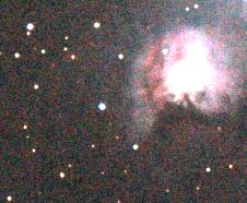
The small part below shows the image before and after filtering of the noise of the red component:

13. How to correct the optical distortion?
Thanks to the big size of the sensors, the images coming from digital cameras are some time affected by the optical distortion problem. In extreme situation the registration is not possible. The example below is a particularly delicate case to process.
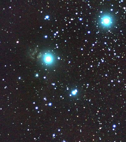
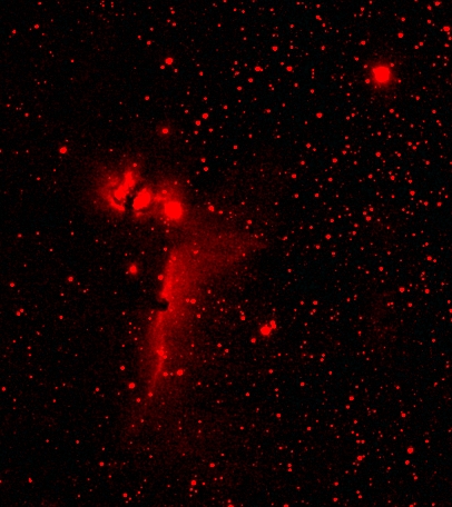
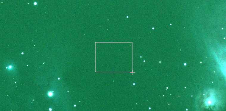
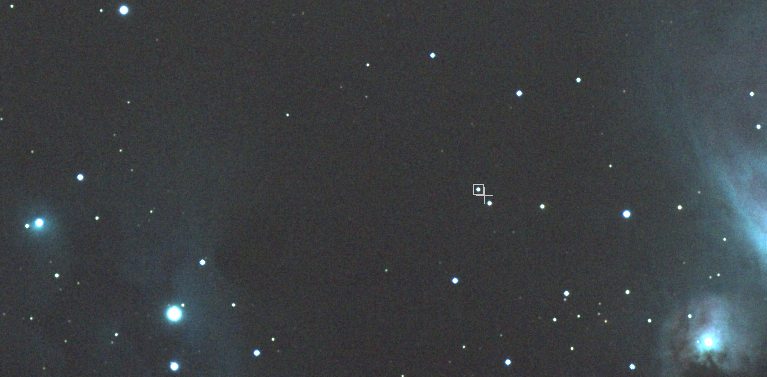
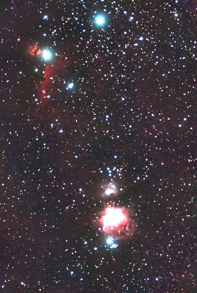
These images were acquired with a teleobjective lens of 200 mm focal focal length at f/4 and a EOS 10D. The observation conditions are those of a sky of city very polluted by parasitic light (limiting magnitude with the eye of 3). On left we have a colors composition of the Horsehead nebula region in the constellation of Orion. It is the combination of 7 frames exposed each 90 seconds, so the total cumulative integration time is of 10 minutes approximately. It is only a part of the original image. Note how the sky was so luminous that the image is saturated by the sky background in only 140 seconds! No color balance was applied, except the equalization of the background for the three layers with the assistance of the BLACK command). On right-hand side, the same field observed with the same instrument, but while adding in front of the objective a red filter Lumicon H-alpha (click here for an analysis of the transmission of this filter associated with the EOS 10D). We have stacked here 20 frames exposed each 280 seconds (total exposure of 1H30 approximately). Only the red layer after conversion of RAW is preserved, the green and blue components being very pale because of the use of coloured filter.
The idea is to add to the component R of the image of left, the "H-alpha " image line in order to have a natural star field in which nebulas appear clearly. The problem is that the filter used is not perfectly flat, which gives a very slight additional optical power to the photo objective and causes especially a differential of distortion between a frame taken with the filters and a frame taken without the filters. The difference in scale makes impossible the superposition of the images in any point of the field (it is lacking some 6 pixels of 7 microns in the worst case, which is not acceptable).
For despite everything it is possible to make a success of the compositage. For that it is necessary to correct the distortion of one image compared to the other. Here how to proceed under IRIS.
If linear default of registration between the two images exceeds 5 to 6 pixels it is recommended to make a pre-centring at least in a point of the image (the center). Use for this the (L)RGB... tool of View command (this command makes it possible interactively to make translation of an image compared to the other).
Load one of the color component, G image for example. From the Analyzis menu, mark the Select objects item. The mouse cursor takes the aspect of cross. Click in the center of approximately 20 to 30 stars distributed well on the whole of the image (not forgetting the edge of this one):
In the console to type the command:
DISTOR IM1 IM2 3
with IM1, the reference image name, IM2 the image which will be deformed to superimpose itself on IM1 (for example the H-alpha image), and finally, 3 is the the polynomial degree of the polynomial function, a generally satisfactory value. When the program completes its calculation, the image which appears on the screen is the IM2 modified image (for other examples of use of the powerful command DISTOR, click here). Finally add the R image and H-alpha image (use ADD command for example). Here the result:

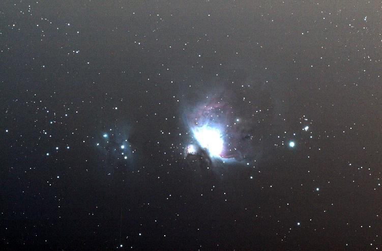
The image below shows practically the complete field observed with the teleobjective of 200 mm and the CANON EOS 10D.
Page (3/3)
|
|
|

