LISA
spectrograph: Variations
about instrumental response
We show in this page the parameters that influence the instrumental response of LISA spectrograph. It supports the demonstration by practical examples.
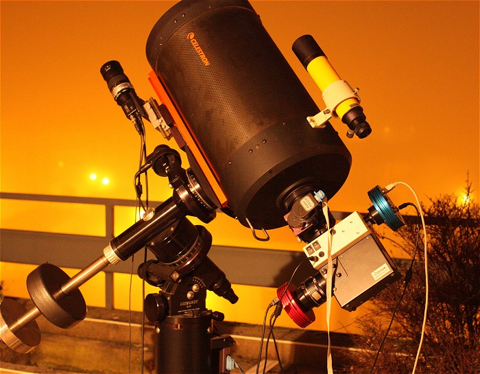
The
setup used. The spectrograph is attached to a C11 telescope (D =
0.28 m). The acquisition camera is a model Atik314L +.
The importance of focal reducer
To convert the F / D ratio of the telescope from F/10 to F / 6 (nearly) - recommended to operate the spectrograph, I use a focal reducer Alen Gee MarK II (BaaderPlanetarium).
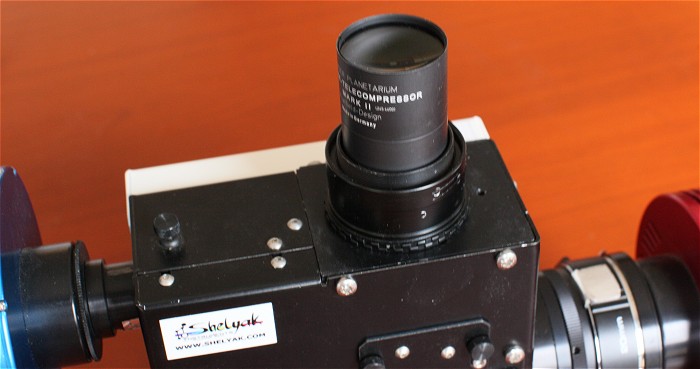
The
focal reducer is the ierface between telescope and IRIS spectrograph.
Like most focal reducer, the Alen Gee is a simple achromatic doublet. The graph below shows variation of best focus poistion along optical axis relative to wavelength for a typical doublet. The horizontal axis represents the value of the defocusing (in microns), the vertical axis represents the wavelength (in microns).

Longitudinal chromatic aberration of a doublet lens.
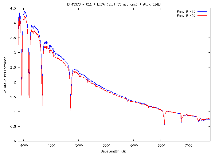
The selected focus plane determine the amoung of wavelength transmited through the slit. This causes a radiometric error. The image below shows how changing the shape of the 2D spectrum relative to focus (we choose positions A, B or C - see preceding figure).
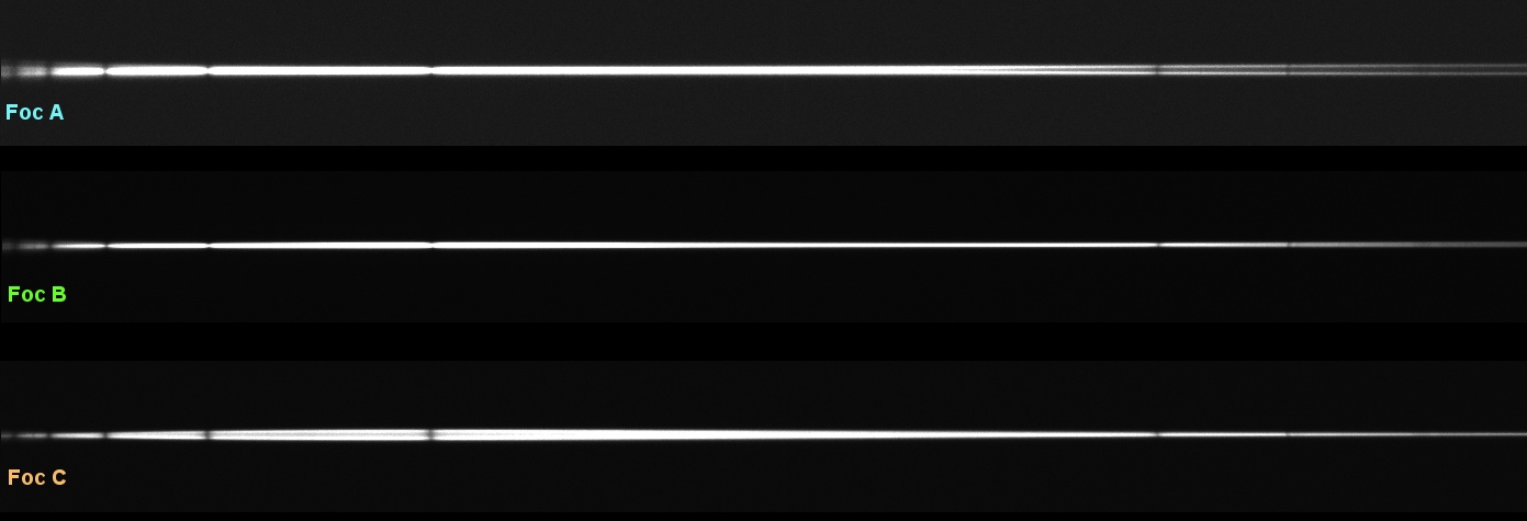
Aspect of HD43378 spectrum (spectral type A2V) function of selected focus.
The focus plane noted "B" is probably the best compromise. Its egalize the focus of red and blue and simultaneously, it maximizes the average flux entering in the spectrograph.The most critical issue here is that the incoming flux depends of the wavelength, hence photometric errors, as shown in the figure below:

Change of observed spectral profile in fonction of focus on the entrance slit. The focal reducer is the Alan Gee reducer. The true profile is probably the green curve.
The focus default in
this demonstration is very high for the demonstration, but this
example shows that it is crucial to effectively monitor this setting
for obtain spectrophotometric qualities. It is important not to
do: adopt a focusing plane when evaluating the instrumental response
of a reference star,then adopt a significantly different focus then
observing the stars of the program. The shape of the continuum is
then biased.
The following figure shows the characteristic
variation of the continuum for two successive focus assumed satisfactory
using the reducer Baader. It is difficult todo much better with
this equipment.
Characteristic variation of the continuum due to the sensitivity assessment of the best focusing plane by associating an Alan Gee focal reducer to a spectrograph at LISA.
One can search best qualities reducer: triplets of lens, apochromatic, .... But these are rare and expensive products. Given what is said above, if one search an absolutely high precision spectrophotometric (this is not always useful, depending on the type of work referred in stellar spectroscopy), a good idea is ultimately to remove the focal reducer. Working directly on the telescope are greatly reduced perturbation induced by the instrumental chromatism. This is the case in a natural way if the telescope is Newtonian, probably the ideal setup with LISA if the primary mirror is open between F/5 and F/8. Good apochromatic refractors in the same range of the aperture ratio are also a good choice. Work without focal reducer with most Schmidt-Cassegrain telescopes is equivalent to a F/10 entrance optical beam into LISA spectrograph. The penalty is a loss of efficiency in the flux can be estimated from 50 to 100% depending on the seeing and the quality of guidance. By cons, the telescope appears much more achromatic. In addition, the optical aberration of the internal LISA spectrograph are reduced and it is possible to attain power maximum resolution of the instrument, say R = 1200, with good uniformity quality between 3900 A and 7400 A (15 microns slit).
Let's see what becomes the instrumental variability response function related to the focus if you do not use a focal reducer (C11 at F/10).
Work without a focal reducer
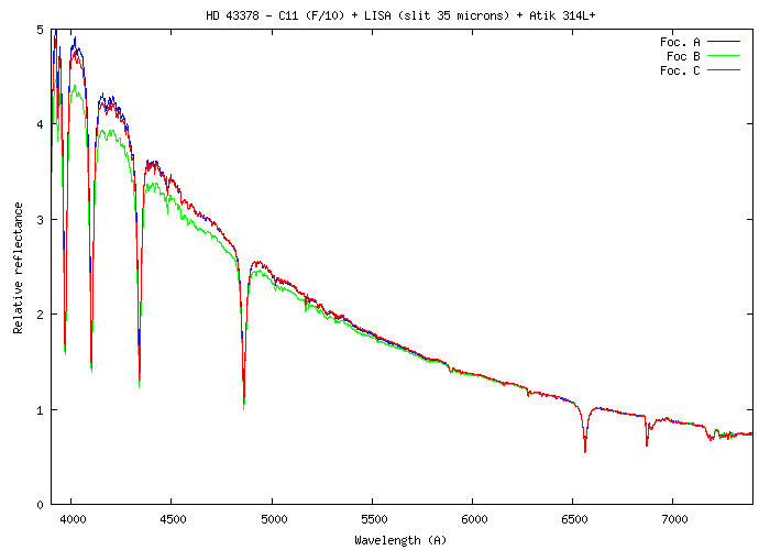
In the 2D spectrum of the star HD43378 below, the effect of defocusing results is an enlargement of the spectrum trace, but unlike the previous situation the trace is significantly more uniform as a function of the wavelength. Chromatic aberration is therefore reduced, especially as it is now working F/10 (tolerance to defocus is higher).

Intra-focused, focused and extra-focused spectra of star HD433378.
Here the corresponding spectral profiles:
Specral response funtion of focus on the entrance slit without focal reducer..
Two successive random refocus sample spectral profile (foc #1, foc #2) compared to the HD43378 Miles profile extracted from ISIS data base:
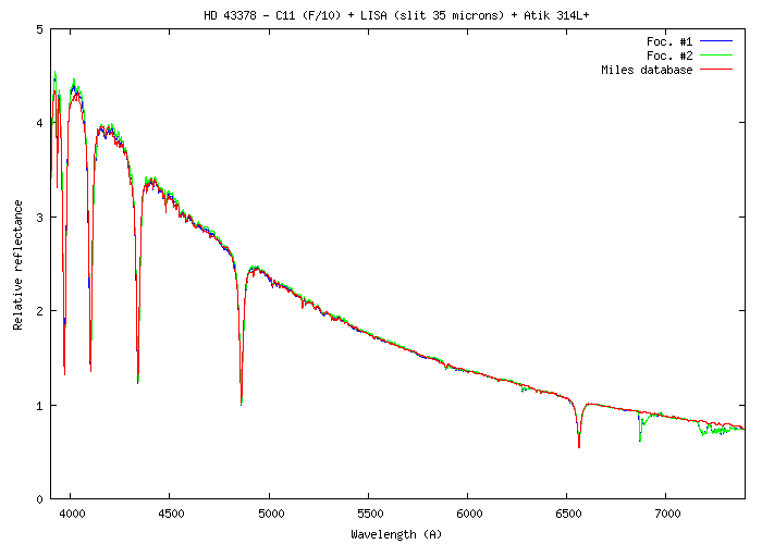
Result of two independants focus (#1, #2). In red, the HD43378 spectral profile coming from the Miles base, selected for find the instrumental spectral response.
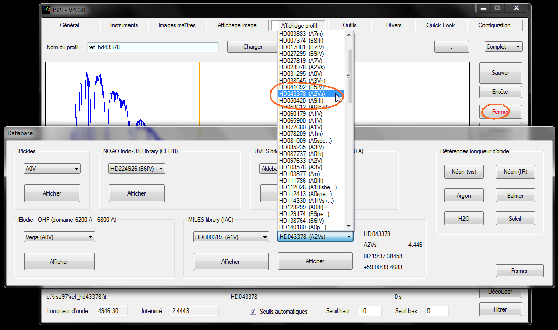
How to extract the HD 43378 profile from MILES library.
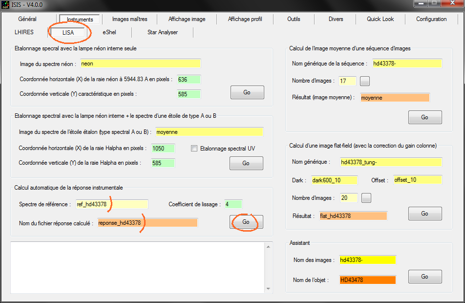
ISIS offers a powerful tool to calculate the spectral response of LISA spectrograph. When you click the Go button, the software firstly process all your your sequence (here the spectra of the star HD43378). This star is called "reference" because we know also the theoretical spectrum (named here ref_hd43378). This spectrum is from the MILES library, but ISIS offers many other choices. For complete processing, ISIS act as you click the Go button located in the "General" tab. This is why the "General" tab should be properly informed. In a second step, the processed spectral profile is divided by the theoretical profile of the star. The result start to resemble to the instrumental response, but ISIS continuing operations automatically by eliminating the main spectral lines of your star and smoothing the profile. In the example, the result is the response file instrumental "reponse_hd43378". You can see immediately the by open the "View Profile" tab.
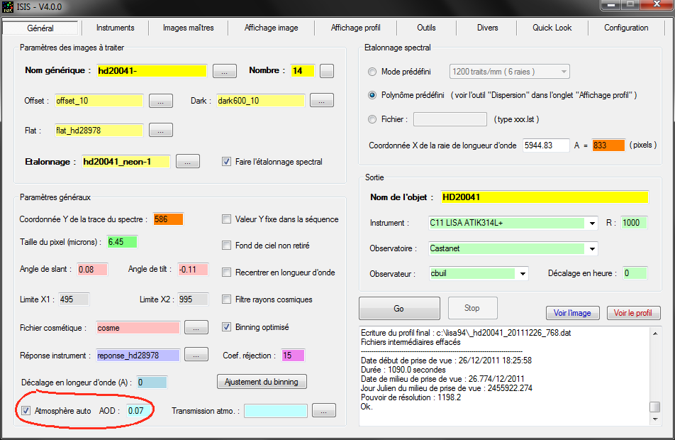
Take into account atmospheric transmission
below (see screen copy) we decide to include the calculation of the transmission during the reduction of the spectra. We uses the ability of ISIS to automatic query SIMBAD to retrieve the equatorial coordinates of the star piped treated (here the object HD20041) and then calculate the angular height of the star, and finally the transmission of
the corresponding atmosphere. Note that you must supply the index AOD (Aerosol Optical Depth), which measures the amount of dust suspended in air. The night was clear and well correspond to the winter season. An AOD of 0.07 is a correct answer.
Last key point: if you check the Auto Atmosphere, for process the stellar spectra (which is recommended), if ou decide to take into accound athmopsheric transmission remenbr to check also the option when you evaluate the instrumental response from a reference star with a known spectrum (here the reference is the star HD28978 - type A2V - coming from MILES library):
As an application,
the plot below shows a sequence of spectra acquired during
the same night (December 26, 2011). The instrumental response is
built on the basis of expected spectrum of the star HD28978. The
AOD index chosen is 0.07 (typical value for the winter and a very
clear night as seen above). In the graphs, the spectrum observed
is in blue, while in red, one finds the expected spectrum extracted
from the MILES library (spectra reddened by intrestellar extinction
in version 4 and beyond). The spectra were acquired with a 19 microns
slit width and a C11 telescope used at F/10, so we favor the
spectral resolution (close of 1000 here) and improve the photometric
quality (no focal reducer).
|
|
|
|
|
|
|
|
|
|
|
|
|
|
|
|
|
|

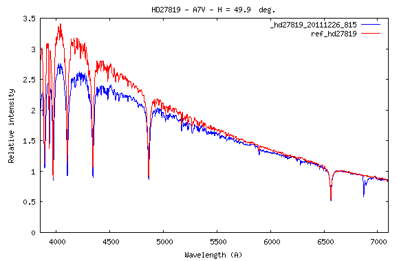
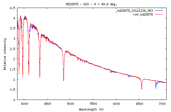


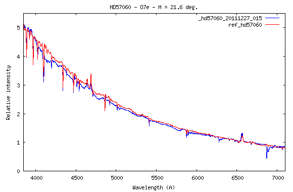
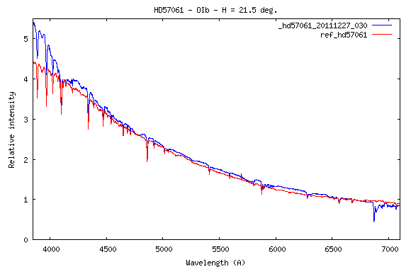
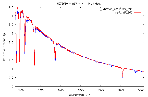


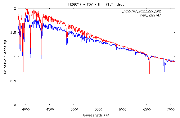
The agreement is quite satisfactory. However, we note a fairly systematic underestimation of the continuum in the blue relative to red. Perhaps this come from the spectrum of the star selected as a reference (HD28978) which may be bluer than shown MILES? Taking into account the atmospheric transmission does not seem concerned (in winter the AOD index AOD is quite low and the curve of atmopsheric transmission are dominated by Rayleigh scattering, which is very deterministic). The choice of star HD31295 as a reference might be more opportum to reduce the median error. It remains to be investigated, but the subject is difficult. The assessment of good continuum of a star is definitely a delicate art.
Incidentally, the graphs presented above were drawn from the free software Gnuplot run directly from ISIS:

Example of two profiles drawing mode.
The spectral flat-field
Although this is optional, it is strongly recommended to pocess spectra wiith ISIS by providing flat-field image:

It is an important conditon for removals possible umbra os dust in the path, the irregularities of the slit width or to correct the interpixel difference response (called PRNU, i.e. Pixel Response Non Uniformity).
The screenshot below shows a typical flat-field images taken from a sequence acquired with the LISA internal white light (tungsten). Here, the slit is 19 microns wide and note also the exposure time (20 seconds). This time is adjusted so that the maximum level in the flat-field does not exceed about 58,000 ADU (cameraAtik314L +). Taking a safety margin against the maximum level possible (65535) to be sure not to saturate the detector and limit possible non linearity errors.. Note again how in the example are named flat-field images (the pricessed star is HD43378). I always use this method. Note finally that it is not mandatory to acquire a sequence of images "tungsten" for each observed object, because it is a lengthy procedure. I do at least one flat-field per night and more if the pointing direction of the telescope change largely for take account of bending of the instrument (mecanical flexure).
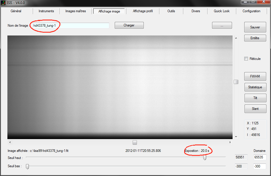
Display of image HD43378_TUNG-1 (_TUNG extension is added to the time of acquisition to easily locate images of this type on the hard disk, as I use_NEON extension for the spectra of internal neon). For a high-quality flat-field end (especially in the blue, where the flux of the lamp is low) it is important to averaging many images of this type, typically 15 to 20 or more.
We use a specific tool tab "LISA" to determine the flat-field acquired with the internal white light (the calculation eliminates all the vertical gradient). Also remember to use the wizard that most pre-filled fields, including the "General" tab. It's convenient and errors risk are reduced:

The actual calculation of the instrumental response is automated:
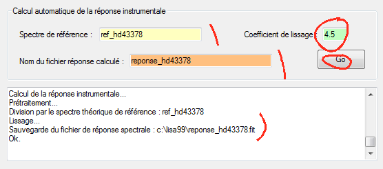
However, it must make a choice of manual smoothing coefficient, which demands attention. The procedure is trial and error by doing a good compromise. The figure below shows how changing the shape of the response function with the coefficient (the values may change, depending on the type of spectrum and nature of residual noise). Each time, go to "Display profile" tab for appreciate the result:
|
|
|
|
Coefficient
= 0,0 |
Coefficient
= 0,5 |
|
|
|
|
Coefficient = 4,5 |
Coefficient = 15,0 |
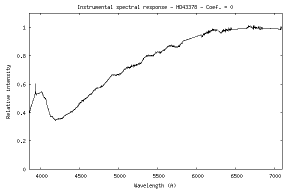
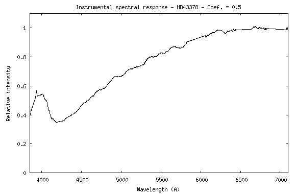
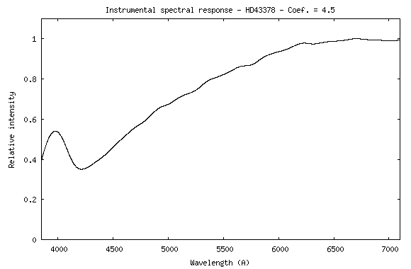

In this example, with no smoothing (zero value for the coefficient), noise and artifacts are present. These structures do not characterize an instrumental response type. With a coefficient 15, smoothing is excessive: the actual response curve is not properly adjusted, especially around 4000 A, where it is rapidly evolving in my LISA. We choose finally the value of 4.5, intermediate:
LISA response with the aid of theoretical and observed spectra of a star (HD43378). The flat-field is here produced by using the internal LISA white light.
We can note a bump around 4000 A. It is actually the result of an instrumental absorption that occurs in the optical calibration channel for the blue-green region of the spectrum.The accident in this region is a source of potential error in evaluating of satrs continuum (because the responsivity of calibration source varies quickly and are therefore sensitive to instrument deformation - gravity effect - for example). Some LISA spectrographs do not have this specail structure at 4000 A - it is not the case for my proper spectrograph.
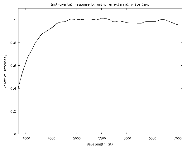
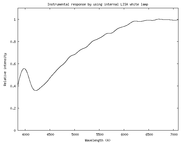
You can also choose to use an external light spot:
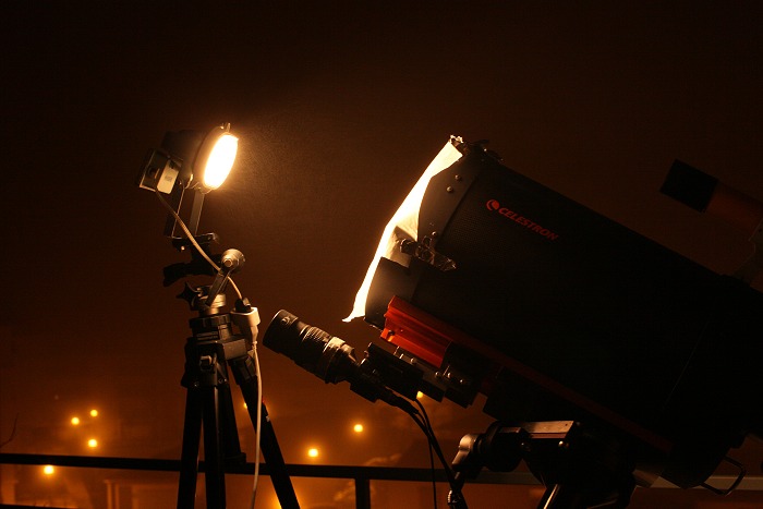
The telescope pupil is now illuminated by a halogen lamp. The entrance of the telescope is covered with a layer of diffusant paper. Under these conditions, the instrumental response curve instrumental is much more homogeneous (results below - remember, the instrumental response is not independent at this stage of the source spectral containt). In return, the acquisition process is notoriously complex and the orientation of the telescope can affect precision due to differential flexure relative to stellar observations. Notice I still tried to limit this mechanical problem (modest with LISA spectrograph) by ensuring that the telescope is up pointing.