Design a classical spectrograph
We are going to calculate a set of parameters for a traditional spectrograph using a reflective diffraction grating, a collimation lens and a photographic objective lens. The detector is a CCD. The desired resolution is about 3000. The results are presented here, along with some usable reductions techniques.
1. Specifications
2. Choosing a grating
3.
Choosing a diffraction angle
4.
Determination of the focal length for the collimation lens
5. Determination of the focal length for
the camera optic
6. Effective spectral resolution
7. Spectral range
8. Optical transmission
9.
Spectrograph's sensitivity
10.
Signal expressed in electrons
11.
Signal to noise ratio
12.
Building and tuning the spectrograph
13. Some typical results
14.
Extracting the spectral profile
15.
Spectral calibration
16.
Frequent lines in stars' and nebulae's spectra
17. Radiometric calibration
18.
Characterization of the line profile
This spectrograph is typical for studies fines structures in stellar spectra, like variations in line spectral profile of Be stars for example. A good target is to determine gas movements in these stars' circumstellar disk with a precision of some 20 to 100 km/s, using the H-alpha spectral line at 6563 angströms. In Be stars, radial velocities of several hundreds of km/s are often observed. In most cases, spectral lines will be just correctly resolved if a radial velocity dv of about 100 km/s can be detected.
To this end the spectrograph's resolution power R should be:
R = l/dl = c/dv
where c is the velocity of light (c = 3.105 km/s).
We need almost for this studies : R = 3.105 / 100 = 3000, or a spectral purity (i.e. spectral resolution) of dl = 6563 / 3000 = 2.2 A minimum. So, our spectrograph model for this description is now named R3000 spectrograph.
Note that if R<1000 the spectrograph is said to be of low resolution. If R is higher than 1000 but lower than 5000 the spectrograph is of medium resolution. For R > 10000, it is said to be of high resolution.
Our spectrograph should be compact enough that it can be mounted on the telescope itself, thus avoiding the transmission losses implied by an optical fiber, a well known source of efficiency losses. It is targeted to telescopes in the 200 mm class and should give access to stars to the 8th magnitude with a signal to noise ratio of 20.
To ease its operation, no entrance slit will be used, thus avoiding the difficult problem of positioning the star's image in the middle of a slit a few microns in width. As a consequence, the usability of the spectrograph is optimal, as well as its photometric efficiency (no loss in stellar light is due to the slit's edges). On the other hand, the spectral resolution is directly constrained by the size of the star's image in the telescope's focal plane, which should be as small as possible. Hence the telescope shall be of good quality as weel as its mount. Moreover, the absence of a fine slit makes spectral calibration of the spectrum complex and difficult. This aspect is not really critical for our purposes, since the spectral dispersion is easily and precisely known. It has been experimentally shown that one can use as a spectral standard telluric lines that happen to be in large numbers around the H-alpha line. This technique allows a level of precision in spectral scaling that makes our spectrograph usable in measuring absolute radial velocities, e.g. for the study of spectroscopic double stars.
Note that the slitless spectrograph should be capable of obtaining both medium-resolution spectra and monochromatic images of moderately extended objects (i.e. planetary nebulae).
Note also that a large entrance slit may however be placed at the telescope's focus (some millimeters of wide). Its role would not be to define spectral resolution, but rather to reduce the sky's background level.
The CCD camera uses a KAF-0401E so it has a good efficiency and allows studies of spectral lines profiles at wavelength below 4000 A (access to the H et K lines for CaII). We will use an AUDINE camera with 1x1 binning (the pixel size is therefore 9x9 microns).
Last, our cost estimate is in the order of $350 for a cheap instrument (without the CCD camera, whose cost is about $1100 for an AUDINE).
For the following numerical application we will assume the telescope is 190mm in diameter with a focal length of 760 mm (F/D=4).
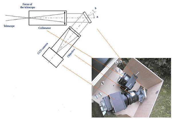
The R3000 spectrograph's optical scheme.
Edmund Scientific is probably the most interesting source for gratings. They have a large choice of components of superior quality at moderate prices.
Since the spectrograph should be light and compact, it appears that the optics' focal length should be fairly short. In order to reach the desired resolution we will have to choose a grating with a large number of groves per millimeter, that is one with a large dispersion power. In Edmund Scientific's catalog we will consider those with 1200 grooves/mm.
The low cost objective makes us choose a medium
size grating, at : 30 x 30 mm. The blaze angle is chosen so most
of the energy can be found in the visible part of the spectrum (around
500 nm). The final choice is a grating referenced E46.077, whose
cost is 96$ (exclusive of shipping costs) .
3. CHOOSING A DIFFRACTION ANGLE
So as to best use the engraved surface of the grating, making sure the beam does not overflow its dimensions, the incidence and diffraction angles should be carefully chosen. Ideally, one should use small angles (this is the Littrow arrangement), but this leads to technical non-feasabilities because of the mere size of available collimation and camera lenses (see the spectr'aude project for a Littrow arrangement).
For our spectrograph we have chosen (arbitrarily in the beginning) an angle between the incident beam and the optical axis of the camera lens of 28.5° (angle a+b in the previous figure). With a 1200 grooves/mm of this size, it is not recommended to increase this angle because vignetting may appear (see further on).
The fundamental grating's formula that gives the diffraction angle b as a function of the incidence angle a is:
(1) 
where l is the wavelength in mm, k the order of the spectrum and n the number of grooves per millimeter. For the spectrum's central wavelength we choose the hydrogen's H-alpha line at 6563 A (or 0,6563.10-3 mm). Also, n is 1200 in our example.
We take into consideration the constraint : a - b = 28.5°.
We can determine the value of angle b as a function of angle a for the cases : k=1 and k=-1 (the selected grating can only work correctly for orders +1 and –1, and anyway it is not possible to use higher orders because incidence angles become too high and the size of the grating is found to be too small). To this end we compute:
(2) 
By successive approximations, the following couples of angles are found:
for k = +1, a = 38.2° and b = 9.7°
for k = -1, a = -9.7° and b = -38.2°
Further on we will see that the spectral resolution is maximal if the absolute value of the diffraction angle b is less that the absolute value for the incidence angle a. Hence we chose the k=+1 solution.
To summarize we have :
a = 38.2°
b = 9.7°
a - b = 28.5°
Note: For another useful equation set, click here.
4. DETERMINATION OF THE FOCAL LENGTH FOR THE COLLIMATION LENS
The collimation lens' role is to project to infinity the image of objects appearing in the telescope's focal plane. When choosing this lens, it is essential to avoid any dimensional overflow of the grating by the collimated beam. If this were to happen the telescope's aperture would be reduced, which would imply a loss of light flux.
The optical beam's diameter measured in the collimator frontal plane (perpendicularly to the optical axis) is given by :
(3) 
with D the diameter of the telescope's primary, F the telescope's focal length, f1 the collimatior optic focal length.
Diameter d1 should be constrained so the beam does not overflow the grating. If L is the grating's dimension seen in the collimation lens' plane and W the grating's physical dimension, then we have :
(4) 
With W = 30 mm and a = 38.2°, one finds L = 23.6 mm. This dimension is an upper limit if we do not want to reduce the telescope's aperture.
Using equations (3) and (4) together we write :
(5) 
which implies that the maximum collimation lens diameter is such that

or : f1 < (760 . 30 . cos 38.2°) / 190 = 94.3 mm
A 90 mm F.L. @ F/D=2.5 Tamron photographic lens was available: it perfectly fits our optical arrangement.
Using formula (3) we find that the effective diameter for the beam is (190 . 90) / 760 = 22.5 mm. By comparing this with L, we find there is a construction margin of 23.6 - 22.5 = 1,1 mm. The grating shall be positioned carefully in front of the collimation lens. We verify that a grating with 30 mm on a side fulfills our needs, but that a 50 mm grating would allow a larger tolerance. Such a component is available with Edmund Scientific, though at a higher price (US$ 142.35).
Last it should be verified that the collimation lens as a f-number enough that the beam from the telescope is not vignetted. The pupil diameter for the selected lens is 90 / 2.5 = 36.0 mm. Since the beam exiting the collimation lens has a diameter of 22.5 mm, there is no problem using our lens. Generally it should be verified that
(7) 
Note that these formulae are valid only when a ponctual object is observed. If one wishes to make the spectral image of a wide object, it is necessary to take into account the pupil imagery. Ideally, it is necessary to conjugate the telescope pupil on the grating through the collimator lens. In your case, since the Cassegrain telescope optics create an entrance pupil at the telescope secondary, the collimator makes a pupil which is about 112 mm from the collimator. This is the nominal position for the grating for cancel vignetting. Remember the following equation: if s is the distance between the telescope secondary and the collimator, if f1 is the focal length of the collimator lens, then the distance s' between the collimator and the grating must be approximately
(7') 
s' = (90 . 460) / 460 - 90) = 112 mm
As a summary:
f1 = 90 mm
d1 = 22.5 mm
s' = 112
mm
5. DETERMINATION OF THE FOCAL LENGTH OF THE CAMERA OPTIC
The spectrograph's spectral resolution will partially depend on the camera lens' focal length.
Let dl be the smallest spectral element that must be isolated in the spectrum. Our specification implies a resolution R=3000. By definition we have :
(8) 
We compute the reciprocal linear dispersion P, usualy given as angstroms/mm, at the camera lens' focus. This parameter is also called plate factor :
(9) 
Sampling theory (Shannon's theorem) implies that in order to resolve a dl spectral element it is necessary that it be sampled by two pixels or more. In other words this means that a spectral interval dl shall be covered by at least 2 pixels. If h is the sampling factor we have h > 2 and the inverse spectral dispersion in A/mm that guarantees there will be no undersampling of the spectrum is:
(10) 
with e a pixel's dimension.
Plate factor expressed in A/pixel is thus:
(11) 
From (8) we find dl = 2.2 A for the H-alpha line, whence the minimal inverse dispersion for no undersampling (equation (10)) :
P < 2.2 / (2 . 9.10-3) = 122 A/mm
or, using (11), P < 1.1 A/pixel.
By relating (9) et (10), we deduce the camera lens' focal length :
(12) 
whereas f2 should be larger than 67.2 mm. We used a commercial photographic objective of F.L. 80 mm @ 1.8 (an used Pancolor by Carl Zeiss Jena found for $100). It has the closest F.L. to 67.2 mm that we had access to. With this lens reciprocal dispersion is found to be (9) :
P = (107 . cos 9.7°) / (1200 . 1 . 80) = 102.7 A/mm, or 0.924 A/pixel.
Following (11) we deduce the sampling factor :
h = dl / P = 2.2 / 0.924 = 2.4
It is slightly higher than necessary, but by experience we fill it is a good thing.
As for the collimation lens, we must check that the camera lens causes no vignetting of the optical beam. As a first approximation the beam's diameter out of the grating can be computed as (for pointlike source):
(13) 
where r is a parameter called anamorphic factor whose values is:
(14) 
We find r = cos 38.2° / cos 9.7° = 0.797.
Diameter d2 can then be calculated using either formula (13) or (14). The result is d2 = 28.2 mm. The camera lens' aperture should be larger than this figure. We verify that this is the case since the pupil's diameter is 80/1.8 = 44.4 mm.
But beware, the value for diameter d2 computed using formula (13) is only exact for a monochromatic beam whose image would focus at the CCD's central point. Things become complex if one tries to collect, with the chamber lens, all of the rays diffracted by the grating that reach the CCD's usable surface. To avoid vignetting at the CCD's edges the chamber lens should be large enough that it can receive the polychromatic beam corresponding to the CCD's spectral range. Thus its dimension should be larger than :
(15) 
where T is the distance between the grating and the objective's entrance pupil (approximated by the lens' front surface) and X the linear dimension of the CCD along the dispersion axis. Obviously there is some interest in bringing the photographic objective and the grating together, but this is sometimes impossible because no sufficient room is available. In our arrangement T could not be less than 105 mm. With a KAF-0401E CCD we have X = 6.9 mm (768 pixels 9 microns on a size each). Consequently :
d2' = 28.2 + (105 . 6.9) / 80 = 37.3 mm.
The Pancolor lens has a pupil diameter of 44.4 mm, which implies that there is no risk of vignetting in any part of the spectrum. However, it must be remembered that the optical lens should be as fast as possible.