6. EFFECTIVE SPECTRAL RESOLUTION
In a slitless spectrograph the effective spectral resolution depends on the diameter of the stellar image at the telescope's focus. The image spot's spreading may be due to turbulence, to tracking errors during the exposure, to optical aberrations, etc. We will use the generic term "seeing" for the angular dimension of the star after a long exposure (more precisely, it is the half maximum width of the stellar image) . If FWHM is the half height width in pixels of the image spot, and we consider that the spectrum has been correctly sampled, we can write that the effective spectral separation power computes as :
(16) 
where P is the dispersion expressed in A/mm, r the anamorphic factor, e the pixel dimension in mm and FWHM the half maximum width in pixels of a star at the telescope's focus.
We note that in order to maximize the spectral resolution it is necessary to have an anamorphic factor smaller than 1. This is what justified the choice of order +1 in paragraph 3.
The typical width at half maximum for the image spot at our telescope's focus is in the order of 2.1 pixels. Thus :
dl = (2.1 . 9.10-3 . 80 . 0.797 . 102.7) / 90 = 1.4 A
According to formula (11) we compute the sampling factor in these conditions :
h = dl / P = 1.4 / 0.924 = 1.5
It appears that we are violating Shannon's
theorem if a resolution of 1.4 A is reached de facto. In practice,
the resolution is somewhat smaller because we did not take into
account the aberrations of the dioptric optics used in the spectrograph
(collimator and camera optics). All in all, an analysis of the spectra
obtained with this spectrograph clearly shows that undersampling
is the cause of a slight degradation in performance (a CCD with
pixels 6 microns on a side should be used rather than one with 9
microns pixels).
The spectral range in Angströms that may be observed in one single image is given by formula :
(17) 
where P is the reciprocal dispersion in A/mm and X the CCD width in mm along the dispersion direction.
With a KAF-0401E (or a KAF-0400) we have X=6.91 mm and since P=102.7 A/mm : L = 710 A
In order to explore the spectral range accessible
to a CCD like the KAF-0401E, from 3000 A to 10000 A, it will be
necessary to rotate the grating by varying the a angle.
The spectrograph's optical transmission is a function of:
t1 = the reflexion factor for the primary
mirror = 0.90
t2 = the reflexion factor for the secondary
mirror = 0.90
t3 = the transmission factor for the collimation
lens = 0.80 (14 optical surfaces with coated optics, reflexion
factor of 0.985)
t4 = the transmission factor for the objective
= 0.80
t5 = the transmission factor of non coated surfaces
(camera and CCD windows) = 0.72
G = grating efficiency = 0.60
(Edmond scientific documentation)
Transmission t is then:
(18) 
The numerical application gives: t = 0.22
In the case where a pointlike source (a star) is observed, sensitivity S is defined as the number of electrons per second and per pixel for an incident flux of 1 photon per square centimeter per second and per Angström at the telescope's entrance:
(19) 
We will now compute near the H-alpha line, i.e. around 6500 A.
We have:
t = optical transmission = 0.22 (see
paragraph 8)
sc = telescope's light collecting area = 238 cm2
(D=19 cm, obstruction of 0.4)
RQE = CCD quantum efficiency
= 0.55 (CCD KAF-0401E at 6500 A)
sp = Spectral range covered
by a pixel (spectrum sampling in A/pixel) = 0.924 A (voir paragraphe
5)
whence S = 26.6 electrons/second/pixel for
a flux of 1 photon/cm2/second/angström.
10. SIGNAL EXPRESSED IN ELECTRONS
We will compute the number C of electrons generated at a point of the spectrum:
(20) 
In this formula C is the number of electrons integrated in an area of Nd . Ns pixels, where Nd is the number of pixels summed along the dispersion axis and Ns the number of pixels summed along a perpendicular to the dispersion axis.
Also we have :
E = star luminosity above the atmosphere in
photons/cm2/s/A.
S = sensitivity as computed in paragraph 9.
Ta = transmission
of the atmosphere. We use a generic value for a sea level site,
Ta = 0.7, which is equivalent to a loss in magnitude of 0.4 with
respect to an observation above the atmosphere.
Tf = transmission
of the spectrograph's entrance slit. Here there is no slit so we
can write Tf = 1.
e
= the fraction of the star's energy integrated in Ns pixels in a
direction perpendicular to dispersion. We will consider that binning
along the transverse axis makes it possible to gather almost all
the available energy, whence e = 1.
Nd = the number of pixels summed
along the dispersion axis. Since we are close to under sampling
the spectrum and we would not want to lose in resolution, there
is no reason to bin along the dispersion axis, and Nd = 1.
The following table gives the spectral flux produced by a star of magnitude 0 and of spectral type A0V (which are the characteristics for Vega) outside the atmosphere:
Wavelength (A) Flux (photons/cm2/s/A)
4000
1620
4500
1453
5000
1167
5500
990
6000
833
6500
700
7000
620
7500
536
8000
483
At 6500 angström the signal for Vega (magnitude 0) will be around :
C(0) = 700 . 26.6 . 0.7 . 1.0 . 1.0 .1.0 = 13000 electrons per second.
Calculating the signal for a star of magnitude m :
(21) 
The computation for a star of magnitude
7 gives C(7) = 21 electrons per second.
If we want to determine whether our magnitude 7 star will be correctly observed for a given exposure time, we must compute the ratio between the signal and the noise (SNR). It is often said that the signal "pops out" of the noise if SNR > 5. In practice, whenever one wants to measure parameters, such as spectral lines' morphology in the spectra for Be stars, the necessary SNR is higher. We will consider that a spectrum will be usable for SNR > 20 (at the continuum level).
The signal to noise ratio is given by:
(22) 
and:
Ti = the exposure time in seconds.
C
= the star's signal in electrons/second after vertical binning (on
the axis perpendicular to the dispersion).
B = the sky background
signal expressed in electrons per second and per pixel.
D =
the thermal signal expressed in electrons per second and per pixel.
Ns = the number of piwels summed along the vertical axis (either
pixels summed a posteriori or binned during acquisition).
Nb
= the number of pixels binned in the CCD during the exposure along
an axis perpendicular to the dispersion.
Nr = the number of
images that have been summed up in order to reach exposure time
Ti.
s
= the camera's reading noise in electrons = 17 electrons for the
Audine camera.
In an urban site, where the spectrograph's tests have been conducted, the sky brightness is fairly high. It is equivalent to a magnitude R of 16.6 by arcsec2. The corresponding signal as measured by the spectrograph is 40 electrons/second/pixel.
We assume that the CCD's cooling is efficient enough that the obscurity current is close to null, or D = 0.
The Ns parameter shall have a high enough value in order to integrate most of the stellar signal. If FWHM is the transverse width of the spectrum in pixels (along an axis perpendicular to the dispersion), then Ns should be equal to 3. FWHM in order to integrate 99% of the signal. The transverse spreading of the spectrum is around FWHM=2 pixels, hence Ns=6.
We suppose there is no internal binning in the CCD along the transverse axis during the exposure. Hence Nb=1.
A long exposure is divided into shorter ones in order to eliminate any tracking problem that would result in a loss of spectral resolution since there is no entrance slit. We will compute the S/N for a star of magnitude 7 with a total exposure time of 1260 seconds divided into 7 exposures of 180 seconds each.
We have:
SNR = (21 . 1260) / SQR(21 . 1260 + 6 . (40 + 0) . 1260 + (6 / 1) . 7 . 172) = 45
The spectrum for our 7th magnitude star will hence be usable with an exposure of about 20 minutes, which fulfills the aim of our specification.
It should be noted that most of the noise comes from the sky background. In order to improve the situation one should observe under a darker sky, or use a rough slit (a few millimeters wide). If the sky background is reduced by a factor of 2, the SNR increases to 60.
The CCD's reading noise impact is marginal. In this situation, know as "photon noise regime", the exposure time that is necessary to obtain a given S/N ratio is given by :
(23) 
For instance it can be checked that in order to obtain a SNR of 45 with a magnitude 7 star the exposure time will be:
Ti = (452 . (21 + 7 . (40 + 0)) / 212 = 1200 seconds.
For another discussion about SNR calculation
click here.
12. BUILDING AND TUNING THE SPECTROGRAPH
Building the spectrograph we just described took two hours of an evening using wooden planks, nails and two-sided adhesive tape: In the following night the first spectra were taken with the computed maximum performances (see further on)...
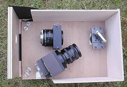
The Medium resolution (R=3000) spectrograph
built to the dimensions computed on this page. Note the 28.5°
angle between the collimation lens' and the camera lens'
optical axis. Both intersect on the grating's surface. Make sure
to set both lenses at infinity: begin with the camera optic and
the CCD camera by targeting a remote object. Then focus the telescope
so you obtain a focused spectrum on the CCD. The collimation lens
is then properly set (the star image comes to its focus).

Settings are not too difficult to achieve;
they can easily be done "by eye". Here one can see the
telescope's pupil (note the central obstruction) after diffraction
by the grating, the eye being located where the camera objective
should be.
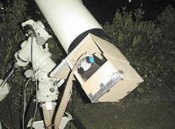
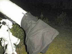
The spectrograph has been installed
on a 190 mm telescope (flat-field-camera 4.0/760 SCL Lichtenknecker
on a Takahashi NJP mount). It is important to get rid of any stray
light: a black cloth should do the trick.