3. TEST OF THE LOW RESOLUTION VERSION
This low resolution spectrograph includes primarily a reflective grating (Edmond Scientific) of 600 lines/mm of 30 mm with used in Littrow assembly and a photographic objective of 35 mm focal length (Nikon F/2), being used at the same time of collimator and chamber objective. CCD Camera is an Audine equipped with a Kodak KAF-0401E. Spectral dispersion is 4.0 angströms per pixel (pixels of 9 X 9 microns).
The preprocessing of the spectra was carried out with Iris and the exploitation with the VisualSpec of Valerie Desnoux.
For the tests the spectrograph is mounted back of Takahashi a FSQ-106 refractor (aperture of 106 mm and 530 mm focal length). Mount is the EM200 model. This equipment is somewhat luxurious and it is clearly possible to work with a more modest hardware. The only parameter to controlling very well is the finesses of stars at the focus of the telescope because the dependance to the final spectral resolution in a slitless spectrograph. If that is possible, it is necessary to reduce the focal length of the telescope (smaller stars), which is very benefit for the resolution. A focal reducer is a useful accessory for F/10 telescopes. It is necessary however to maintain F/D>4 for avoid occult the telescope beam inside this spectrograph.
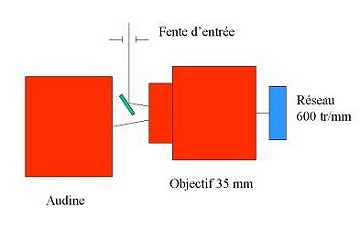

Schematic
diagram and a metal version

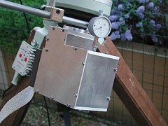
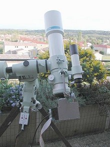
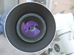
Location of the observation, particularly polluted, in particular by a lighting of sodium lamps. Note the use of the comparator for a precise focusing. The refractor is a quadruplet fluorite giving of very good images, with particularly low chromatism.
The spectra of the low resolution version have a significant curvature and it was necessary to adapt the software for the extraction of the spectral profile to this situation. A specific procedure of calibration will be described further.

Spectrum of the star 54 Oph. The dispersion axis is horizontal and the spectral field goes from 4500A to 7500 A approximately. It is noted that the spectrum is not rectilinear, the radius of curvature being here of 29000 pixels. A special function in Iris makes calculate the spectral profile which takes account this curve (the binning zone is into the two central plot curves ). The most external plot curves delimit a zone in which the level of sky background is evaluated.
A characteristic of this spectrograph version authorize a direct imagery (without dispersion of the light) by directing the grating normal parallel to the optical axis of the objective. By using a broad slit, that makes it possible to identify the field (approximately 10% of incidental flux are then used). It is also possible to exploit this zero order image to carry out the spectral calibration of the spectra, as well as the radiometric calibration (see further). During the tests, this provision it is proven extremely practical and effective (thanks to the adoption of a precise mechanical device for the grating orientation).

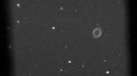
Top, the first order spectrum of nebula M57. Bottom, the zero order image. Note the relation between the position of stars and their spectra. On the direct image it is possible to see vertical contour of the broad slit (not perfectly focused here).
We now evaluate the efficiency of the instrument used - i.e. the throughput. This throughput is the ratio of the number of photoelectrons produced in a spectral element (1 pixel) at a certain wavelength by the number of photons penetrating in the instrument for the wavelength in question.

Total efficiencu of the spectrograph, the refractor and the detector. The atmospheric transmission is also taken into account.
The throughput is maximum towards the wavelength of 600 nanometer and reached 17%, which is a good figure for a spectrograph. The curve was plotted starting from the analysis of the spectrum of the Vega, a type A0V star.
We explain now how to calculate a point of this curve. At the wavelength of 6000 angströms, the Vega produces outside atmosphere a spectral flux of 845 photons/cm2/ s/A (see further one expression for the calculation of this value). The diameter of the refractor is of 10.6 cm, so the collecting surface is 88.2 cm2. Theoretical Input flux in the instrument is (we consider for the moment a transparent atmosphere):
845 X 88.2 = 74529 photons/s/A
The spectral interval in a pixel taking into account dispersion is 4 angströms. Photon flux coming from a perfect instrument in a pixel is then:
74529 X 4 = 298116 photons/s
The exposure used to observe Vega is 1.7 second (beyond, the detector is saturated). In this integration time it thus come on the detector:
298116 X 1.7 = 506797 photons
In addition, one measures after binning that the signal in the image of the spectrum of Vaga at the wavelength of 6000 angströms is of 43213 ADU after 1.7 seconds of exposure. Taking into account the electronic gain of the Audine camera used, which is of 2 electrons by ADU (Analog Digital Unit), one deduces from it that the total number of electrons in pixels at the time of the observation of a zero magnitude star, spectral type A0V and for exposure of 1.7 second is of 2 X 43213 = 86427 electrons.
The theoretical value of the signal calculated upper is 506797 electrons for a perfect instrument, one deduces the instrument throughput (including atmosphere) at the wavelength of 6000 A is 86427 / 506797= 0.17 = 17%.
At this wavelength the quantum efficiency of the CCD is 61%, so the total transparency of the optics (and the atmosphere at the time of the observation) is 28%. The efficiency of the grating used is from 62% at 600 nanometers. So, the remainder of optics represents a transmission from approximately 45%, a figure which one finds well by calculation by taking of account the losses of flux in the various optical surfaces (many because of the use of a photographic objective) and the attenuation of the atmosphere. Note also the availability Excel spreadsheet for facilitate the calculation.
Goto index page Previous page Next page