3.4. Calculation of the signal-to-noise ratio
The following image shows a limiting test magnitude. The star observed (in the field of M57) is of magnitude 10.5. The SNR (signal to noise ratio) measured on the spectral profile is 6 for an exposure time of 9 minutes and the FSQ-106 refractor. The principal; parameter which constrained the detectivity here is the brightness of the sky background, particularly high in the place of observation (limit magnitude to eyes of 3). A less wide slit (about 1 mm instead of the 5 mm current) would have decrease significantly the level of the sky, while maintain the centering of the object relatively simple.
Cumulated
9 minutes exposure of a magnitude 10.5 star.
The signal axis
is expressed here in physical value (in ergs/cm2/
s/A).
We will check by numerical simulation the value of this SNR towards the region of H-alpha to 6563 angströms.
That is to say E0(l) spectral flux outside atmosphere of a magnitude V=0 star and spectral type A0V. The flux is expressed in a number of photons per square centimeter, per second and per angström (or in summary: photons/cm2/ s/A). The numerical value is given by the following formula:
with:

and:
l = wavelength in angström for which one wishes to know the flux = 6563 A (wavelength of the H-alpha line)
T = effective temperature of star = 10800 K (for a A0V star)
BC = bolometric correction = -0,4 (for a A0V star).
Calculation gives E0(6563) = 733 photons/cm2/ s/A.
Consider now N 0(l), the number of electrons per second in a spectral element for a star of magnitude V=0 (the spectral element is delimited by the size of the pixel following the direction of dispersion). We have:

with:
E0(l) = 733 photons/cm2/s/A for l = 6563 A.
S = collecting surface of the telescope = 88,2 cm2 (for the FSQ-106 which has a diameter of 10,6 cm, in the case of a telescope, it is necessary to take into account the central obstruction)
Dl = value of spectral sampling = 4 angströms per pixel with a grating of 600 grooves/mm, an objective of 35 mm focal length and pixels of 9 microns.
Fl = factor of binning in the CCD realised at the reading time along the axis of dispersion. For the tests one did not make a binning in order to preserve the maximum spectral resolution, so Fl= 1.
R(l) = throughput of the instrument which includes the typical atmospheric transmission here, transmission of the optics, the efficiency of the grating and the quantum efficiency of the CCD.
We adopt R(6563) = 0,14 (see figure hereafter).

e = fraction of the total signal of star taken into account at the time of the numerical binning in the space direction to build the spectral profile (binning in the direction perpendicular to dispersion). We consider here that the binning is sufficient broad (7 pixels) to integrate all stellar flux, therefore e = 1.
With the numerical values one finds N0(6563) = 733. 88,2. 4. 1. 0,14. 1 = 436200 electrons/second.
In the case of the observation of a source diffuses (spectrum of a galaxy for example) the signal per unit of time (in electrons/second) is given by:

with E0(l) the surface brightness of the sky (luminance) in electrons/cm2/ s/A/arcsec and:
p = the number of pixel integrated in the space direction (direction perpendicular to dispersion).
Q = the angular scale by pixel according to the space direction = 3,5 arc-second per pixel in the case of the FSQ-106 used with Audine.
W = the angular width of the input slit the spectrograph (in second of arc).
The signal SNR is given by the formula:
with:
Ncont = signal in electrons per second in the continuum for a star of magnitude m. This quantity this deduced from the formula:
Here we have m=10,5, so Ncont= 2,28 électrons/s.
Nsky = the average signal sky background under the spectrum in electrons per second and per pixel. This quantity is raised directly from a long exposure for precise measurement. One finds Nsky= 10 électrons/s for the observatory (very polluted) for a 970 arcsec wide slits and a zone of the image which exclude the significant spectral lines from the illumination (sodium essentially). On the level of the spectral lines of urban lighting the sky signal is 4 times higher.
Ndark = dark signal (or thermal signal) of the CCD in electrons per second. Statistical analysis of images made in the darkness show that the rate of dark signal is of 0,3 electron/seconde under the conditions of observation night.
p = width in pixel of the binning region along the axis perpendicular to dispersion to calculate the spectral profile (number of added pixels). The adopted value (p=7 pixels) is characteristic to integrate all significant stellar flux with the Littrow spectrograph for weak stars.
FS = the factor of binning within the CCD along the space axis (perpendicular to the dispersion). For the tests no intern binning in the CCD was realized, so f=1.
s = reading noise per pixel for Audine camera. We adopt 18 electrons.
T = total exposure time = 540 seconds in our example (stack of 9 one minute integration each one).
N = quantities of stacked images for the total exposure time. Here T = 9.
We have then:
This is the same valeur that the experimental value.
The graphs hereafter shows the magnitude limits reached with various instruments for a SNR on the continuum of 10, sufficient to take some astrophysical measurements and to recognize a spectral type.

Limiting magnitude for a SNR of 10 and a dipersion of 4 A/pixel according to the exposure time (in seconds) in the vicinity of the line H-alpha for a star of the A0V star. The conditions of calculation are: for the FSQ-106, p=7 and Nsky= 10 e-, for the Cn-212 (Takahashi telescope in version Newton) p=10 and Nsky= 10 e-,for T60 (telescope of 60 cm of the Peak of the South) p=12 and Nsky= 2,5 e-,. In all the cases the total exposure time is segmented in 180 seconds elementary poses.

Even condition that above, but for a dispersion of 8 A/pixel by making a binning of a factor two following the axis of dispersion (fl= 2). The gain in detectivity is approximately one magnitude.
An alternative of calculation is to predict the result of the observation of spectra with emission lines. This situation is particularly current with the Be stars and systematic for example in the spectra of novae or quasars. The intensity of the line is then given by the equivalent width W. In a Be star in relatively moderate emission we have W=5 angströms (for H-alpha line quasars one can adopt W=200 angströms, which means very intense line compared to the continuum, and what allows remainder to facilitate the detection of these of objects).
The intensity of the emission line is given by:
Maybe for our star magnitude 10,5, Nline= 2,28. 5 = 11,4 électrons/s
Calculation gives:
Such a SNR on this level of the emission line makes the observation relatively easy for a star magnitude 10,5. Such an emission spectrum is detectable until magnitude 11,5 with refractor of 100 mm only. The performance is still better under a quite black sky and a finer slit (the noise of the city background is the term of noise dominating here).
To illustrate the preceding remarks, the figure hereafter shows the detection of the emission of the H-alpha line in quasar 3C273 carried out with a telescope CN-212 telescope (diameter of the principal mirror of 212 mm). The mirror of the telescope, used in Newton mode with F/D=3.9, was slightly occulted by the spectrograph with an equivalent diameter of 185 mm. The camera is an Audine exploited in 2x2 binning (dispersion of 8 angströms per pixels). Exposure time is of 36 minutes. (add of 12x3 minutes exposures). It should be noted that the sky, in addition to being polluted by the light of urban lighting (limiting magnitude has the eye of 2.5), was clouded with some cirrus at the time of the observation (May 13 2001) ! The wavelength measured of the H-alpha line is 7598 A (measurement is facilitated by the presence in the field of star of magnitude 10,7 which shows quite clear Balmer lines). The spectral shift towards the red is 0,158, which is exactly the value awaited starting from the information of the catalogues.
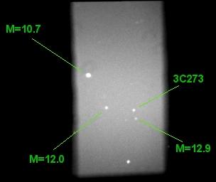

Top, the
field of quasar 3C273 observed in order zero (3 minutes exposure).
Bottom, the spectrum of all the objects of this field. Note that
a star close perturb analysis to the spectrum of 3C273. The continuum
is very weak in the vicinity of the line H-alpha but this line is
quite visible because of its emission. In this image a star of magnitude
12.9 product a readable spectrum. Telescope CN-212 and spectrograph
used with a dispersion of 8 A/pixel. 36 minutes total exposure time.
Date: 13.1 May 2001.
The calibration procedures of the spectra were the subject of a detailed attention during work on this prototype (see chapter 4 for a detailed description). The most delicate part is the flat-field correction (determination on the relative responsity of each point of CCD image). The difficulty in spectrography comes to the fact that a uniform range of light being used to illuminate the surface for determination of corrections coefficients has more or less known spectral contents. The flat-field image is thus the product of an image depending on the wavelength (because of the spectral signature of the source and the spectral throughput of the instrument) and of an image depending on the optical vigneting (in this last term we include also the relative variation of sensitivity pixel to pixel). The problem is to separate these two images. Part of the solution consists in using a source of light of well-known spectrum. It is often an incandescent lamp which is used for that, but this type of solution it is proven problematic to implement with the low resolution Littrow and broad slit. A possible reason is a bad baffling into the spectrograph, problem which will have to be solved thereafter (The internal part of the prototype are not painted in black what does not facilitate either the radiometric calibration because of the present stray light reflections). In the final analysis, the procedure which gave the best result consists in use of the zero order image to determine the optical vigneting (the wide of the slit is the same dimension of the CCD chip), then to observe one or more stars of well-known spectrum in spectrograph mode to determine the spectral sensitivity (this last operation is now well know under VisualSpec). The slit of the current spctrograph must be adapted to make possible this operation.
The radiometric procedure of calibration also takes into account the presence of the diffusion within the spectrograph, which creates a term of offset which can be variable according to the wavelength. The diffusion is measured in two masked zones of the slit, on both sides of the opening. The adopted value is the average of these two measurements. Here still, the slit will be modified to facilitate this measure to the future.
The problem of the spectral calibration was also studied carefully. Indeed, the covered spectral extent is such as it is not possible to consider that dispersion is linear (the variation with the linearity reaches nearly 30 A from one end to another of the spectrum). The dispersion low calculated is:
with x is the position in the spectrum in pixel. The parameters a, b and c are given starting from the measurement of 3 know spectral lines under VisualSpec. The error of residual spectral calibration is then lower than 8 A from 4500 to 7500 A for a dispersion of 4 A/pixel.
The coefficients calculated for the current spectrograph are:
a = -1.4426.10-4 ; b = 4.114 ; c= 4470
The term c depends on the position of star in the slit. Average dispersion is 4.00 A/pixel
Concerning the extraction itself of the spectrum profile and the subtraction of the sky background, we saw it, it is necessary to take account of the curve of the spectra. These phases of the processing will be analyzed in the following chapter.
The low resolution version of the Littrow version tested here proves to have characteristics close to the hoped theoretical level. The chromatism of the photographic objective makes is reasonable low between 670 nm and 450 nm. The availability of zero order image is very useful for spectral calibration (10 angströms precision approximately) and field recognition.
From a theoretical calculation using the precedent results, it appears that the low resolution version tested here exploited in a quite black sky and while posing around 20 minutes should reach with SNR of 6 magnitude 15 on C11 telescope and magnitude 16.7 on a telescope of 600 centimeters. This open many prospects. It should thus be possible to follow a good number of variable stars with telescopes of this diameter, including Mira, with for example fine spectrophotometric measurements. Novae could be studied over long periods. It is the same for the observation for comets. Lastly, some supernovae become the possible target of the amateurs with a spectral resolution of 800, very near to what the professionals in the field do.
The principal improvement to be brought to the current version relates to the development of a system of adjustable slit in width. This necessary in the field of some observations, i.e. extended object, a such comet or a planetary surface, for the calibration and constitutes an effective means to eliminate light of city , while keeping the current facility of pointing of the objects. Click here for see a typical narrow slit application (LINEAR A2 observation).
Goto index page Previous page Next page