- Achieving measurements -

Accuracy check provided by your set of reference spots

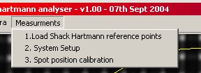
Ok, so now, the first thing that can be done, is to check that your reference spot file is valid. In the next menu click to "1. Load Shack Hartmann reference points"

An open dialog pops up, select the spot reference file.

Once those steps are passed, the reference points are loaded and display over the image as red squares where the center is the reference position. Inside these squares the software attempts to compute the centroid of the spot, provided the rule explained previously (detection is valid when SNBR*Noise+Mean < Max Spot). Always check that some spots are not saturated (max equal to 255) otherwise measurments is jeopardized when spots are satured, avoid also to deal with very faint spots.

Whenever the spot centroiding is computed successfully, a red cross is displayed above the calculated position. One can choose or not choose to combine incoming frames. The violet box indicates the valid point inside the pupil and not inside the central obscuration. 184 spots have been validated within a radius of 217 pixels, where the mean DXDY gap is 0.55, the mean DX gap is 0.02 and the mean gap DY. The mean DY gap is large because my setup making the flat wavefront has shifted a little bit since I've made the reference spot file.

The computation of the Zernike coefficients is automatic and leads to a large Z2 tilt figure that can be deselected. The display box allows to turn on/off the drawing of the wavefront, the PSF. In that case the PTV error is Lambda/12 and the strehl ratio equal to 99.05%. Meaning that a single "noisy" acquisition of the reference points with respect to the reference points gives a very good accuracy. The accuracy is limited in this case by the detector read out noise. While combining frames, the accuracy goes up to Lambda/30 PTV (Microlenses 10 mm focal length). This is the intrisic accuracy of this apparatus (please do not forget to check out X tilt and Y tilt).

By turning on the "Display Elongations, scaled by", show the errors between the last measurement of a spot and its reference. Keep in mind that, in the next pictures, the gaps are scaled by 30x. this is a good tool to detect "non random" wavefront aberrations. In that case the lengths and the direction of the white lines are pretty random. Also the zernike coefficients are all the same magnitude. If one dominates, check what has changed since your reference spots have been acquired. If only Tilts zernikes are involved, just deselect them, if defocus has increased, check focus.

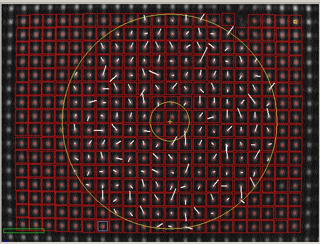
If combined frames is turned on, the gaps are getting smaller and smaller. Nevertheless, some spots, such the one indicated by the yellow arrow, shows a bad trend : larger gap and fixed direction. This spot should be removed either in the list of reference spots, or by reducing a little bit the radius of the pupil.

Measuring a real wavefront.

Example 1 : a star into the sky or a fake star made by an optical testbench.

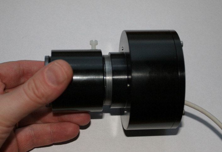
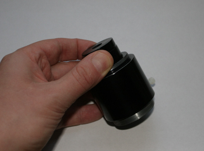
Disassemble first the SH body and collimator holder.

Remove the 5 or 10µm pinhole and replace it by a 100,300 or 600µm pinhole.

This pinhole aims at giving an area where the star will be allowed to be seen by the shack hartmann device.

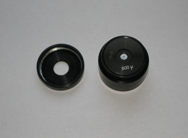
Put the pinhole size mark up ! Avoid to put it upside down !

Install the collimator into its holder

Then before assembling the SH body, install the collimator holder into the telescope (for instance) as if it would be an eyepiece.
Look thru the collimator (like it would be an eyepiece), so that you see the pinhole and the star image sould be inside the pinhole and focused.

If the "star" is visible, its wavefront will go into the shack hartmann device.

Then, at that stage you can screw the collimator holder with the SH body, paying attention that the star does not escape from the pinhole.

Once the SH body is assembled, this pattern of spots can be seen. The circular telescope input aperture is visible, as well as central obscuration.

Video here (notice that atmospheric turbulence is shaking the spots)

In this case, an Intes 180 mm diameter has been used, coupled with a 15 mm collimator.
Since this is a f/10 instrument, a 1.5 mm pupill diameter will be produced at the webcam level (1.5 mm = a radius of 130 pixels).
The central obscuration has been taken into account (radius = 57 pixels). The pupil center has to be set accurately (X=334 and Y=243). The star used was Cappela, the software found 52 valid spot centroid. The wavefront has been reconstructed, and lead to L/2.8 PTV (L/20 rms). Since this is a snapshot, turbulence is also playing a role. Z1,Z2 and Z3 can be deselected, because they don't bring relevant information.

The spots that are included into the pupil diameter and that are outside the central obscuration are taken into account.

The measurments can be turned on, taking care that spots shall be inside red squares.

When centroiding is successfull, a red cross is drawn over the spot. If centroid has failed, no cross is drawn. If some spots are missing, this is not criticial... the software discards them, and computes the wavefront. Keep the spot inside the red square.and keep in mind to avoid saturated spots !

At the end, an HTML file can be generated automatically.

Example 2 : TBD.

Zernikes polynoms

The following table provides the corresponding ZEMAX software zernike polynomial with respect to this SH analyzer indexes.

SH analyzer has the 19 Zernike polynomial that are explained here :
http://astrosurf.com/cavadore/optique/shackHartmann/publis/ih_sh.pdf

R and Teta are polar coordinates, R from 0 to 1, Teta 0 to 2Pi

We have adopted one of the standard coordinate conventions for Zernike polynomials that has Teta=0 along the
y-axis increasing toward the x-axis. The diagrams have +y up and +x to the right.

Piston is not taken into account.

This has been written according to ZEMAX documentation released by Jan 6 th 2003 : the following table provides the correspondance between zernike indexes.

1. means if Ai is a coefficient provided by SH analyzer, it must be multiplied by Factor to get the ZEMAX Zernikes Std polynoms. Sqrt stands for square root of.

PREVIOUS MENU