CCD planetary imaging at under-sampling conditions:
from grayscale snapshots to three-dimensional RGB time-lapse animationsby António J. Cidadão
Well, let's admit it, who has never thought about obtaining a sharp image of the Cassini division on Saturn's ring system, to grab the colors of the Jovian cloudtops or even to show a rotating planet to a group of friends? Well, it's easier than you may think, namely with our modest backyard telescopes, if we choose to use one of the CCD-cameras currently available to the amateur community. But equipment isn't everything. Let's imagine for a brief moment that we planet fans are lucky enough to have access to the best telescope in the world, located at a premium site that allows high-resolution work and, obviously, equipped with a high-end refrigerated CCD-camera. Even with such a dream set-up we would still have to follow one of the most important rules for high-resolution imaging: to chose an appropriate image sampling. Well, this basic rule also applies to our backyard reality. We just have to decide what appropriate means.
This mosaic illustrates the starting point (grayscale original images of Mars, Jupiter and Saturn at the center, all obtained with the ST-6) and the final result (corresponding RGB images at the right) of the image-processing routine I always use to obtain planetary images while working at under-sampling conditions. The Jupiter image at the left is just a blow-up of the initial and final images (4x and 2x enlarged, respectively), here aligned side by side to allow a better comparison between pixel size of the original images (image sampling = 0.75 arcsec/pixel) and the definition that can be obtained after image-processing.
According to the Nyquist sampling criterion, at least 2 pixels must be used to cover the theoretical resolving power of a given telescope. If we use less than 2 pixels to sample the finest details in our images, that is if we under-sample our data, permanent loss of information will occur. For instance, a telescope that resolves 1 arcsec must be equipped with a CCD-camera whose pixels cover 0.5 arcsec. This optimum set-up is reached by working at a correct focal length and by using a camera whose pixels have the most adequate size. The necessary calculations are easily made using this formula F=206xP/S (F= focal length in millimeters, P= pixel size in microns, S= image sampling).
It is common knowledge that the above criterion doesn't have to be followed when imaging deep-sky objects, because local seeing conditions often degrade image quality during long exposures. In practice, the theoretical resolving power of our instrument will never be reached. In contrast, we do know that to choose such an optimum image sampling is of paramount importance when attempting to obtain high-resolution planetary portraits. And it's important since we expect that the short integration times that are commonly used to image bright planets will be able to freeze atmospheric motion and thus will allow us to reach the theoretical resolving power of our telescope.

Optimum image-sampling conditions (2 pixels/0.5 arcsec) for high-resolution work with a 10" telescope are shown at the left (theoretical resolving power of about 0.5 arcsec). According to the variable positioning of a given image point over the CCD matrix, a slightly different image will be produced. It is conceivable that the cross-shaped pixel pattern will be the most frequent, since the square pattern only occurs at a precise pixel/image-point superimposition. Anyway, the dimension of the pixel-pattern and image point closely resemble. This is particularly true if a group of similar images are adequately co-registered and then averaged. The image under-sampling conditions obtained with one of my camera-telescope set-ups are shown in the middle. In this example, regarding the ST-6, it is evident that the best possible image of a 0.5 arcsec image-point will be a 0.75 arcsec square (single pixel). However the resulting pixel pattern can be much more unfavorable when the image-point falls over more than one pixel. As an attempt to partially overcome such problem I routinely use the procedure shown at the right. Original images are first subjected to sharpening and then enlarged 2x with pixel interpolation. While these steps just produce a larger image with pixels still having its original size, it is in practice equivalent to emulate an image of the same size but with smaller pixels (1/2 the original size). Such images can thus be much more precisely co-registered. The final goal is to be able to recover the original sampling conditions in the final processed image, that is to achieve 0.75 arcsec resolution. The theoretical resolving power of the telescope will not be reached but, in my opinion, an improvement in image definition does occur. This approach also applies to the planetary images I obtain with the ST-5C.
Unfortunately it is often difficult, if not impossible in practice, to obey to the above described optimum sampling criterion. For instance, we may own an excellent CCD-camera with large pixels, a camera that we routinely use for deep-sky objects but that we would also like to try on planets. Another possible scenario is that our CCD-camera does have small pixels, but it will have to be used with our small aperture telescope. In both cases, working at longer focal-ratios will determine an intolerable decrease of image brightness. And that will force us to use integration times that are incompatible with local seeing conditions and/or with the stability of our mount. In short, we may eventually reach a proper image sampling, theoretically speaking, but we will be unable to take advantage of it in most of our observing sessions. In other words, we will easily originate lots of "well" sampled albeit blurred images. In my opinion, that's the main reason why planetary imaging has not gained the popularity that its deep-sky counterpart has among the amateur community.
So, what's the solution from my point of view? Well, it's quite a quite simple one: always give priority to short integration times and never mind about having to accept some degree of image under-sampling when necessary. In this article I will describe the procedure I use, and I will try to show some of the results that can be obtained when a group of such under-sampled but sharp images are correctly combined to produce a final image. And you will see that, from such images, the production of stereoscopic-pairs and time-lapse animations is just a few simple steps away.
I presently do all my planetary imaging with a concrete pier-mounted Meade 10" (f/10) LX200 Schmidt-Cassegrain telescope from a "roof-top" observatory located in Oeiras, Portugal. It's a considerably light-polluted urban site, distant about 1km from the ocean and often characterized by poor seeing conditions. Fortunately, some periods of average/good atmospheric stability also occur, and I try to benefit from such occasions to get the highest resolution planetary images that my telescope-camera set-up allows.
Until a last July my telescope was equipped with a SBIG's ST-6 cooled-CCD camera (23x27 micron non-square pixels) plus a CFW-6A motorized color filter wheel, but I now also own a SBIG's ST-5C model (10 micron square pixels; without the internal color filter wheel). For both CCD-cameras I usually add a Meade's Series 4000 2x apochromatic Barlow lens when I want to snap a planet's portrait. For the ST-6 plus filter wheel, my camera-telescope combination provides an image sampling of about 0.75 arcsec/pixel, while for the ST-5C the figure is about 0.4 arcsec/pixel (or about 0.8 arcsec/pixel when the camera works at low resolution; 2x1 binning=20 micron square pixels).
In both cases, the image sampling I adopted is below the optimum set-up for high-resolution work. In fact, taking into consideration that the theoretical resolving power of a 10" telescope is about 0.5 arcsec, I should use an image sampling of at least 0.25 arcsec/pixel. To meet this requirement I would have to work at f/87.5 for the ST-6 (F=22,248mm) and at f/32.5 for the ST-5C, which would be rather unpractical. In fact, the average seeing conditions at my site are incompatible with the integration times I would have to apply. This because I always chose integration times that fill 1/2 to 2/3 of the full-well capacity of my ST-6 and ST5-C CCD-sensors. This way I obtain an adequate signal-to-noise ratio that allows me some freedom during subsequent image-processing.
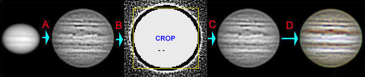
Summary of the sequential processing steps I routinely use to obtain planetary images (see text for details). The image shown at the left is an original red-light frame of planet Jupiter obtained with the ST-6. Steps A to C are performed using SBIG's CCDOPS for DOS software. Step A consists of sharpening, enlarging and resampling the original frame. In step B images are properly cropped in order to become perfectly co-registered. A given number of co-registered images (e.g. 4, 16 or even more) are then averaged in step C. The final red-light image thus obtained can be used as such, but it can also be merged with similar green- and blue-light pictures in order to obtain a true-color RGB image. This final step D is easily performed using image-processing software like Adobe PhotoShop
To partially overcome the limitations imposed by such under-sampling only accepted for practical reasons, I always use an image-processing routine based on a precise sub-pixel co-register of a series of original images that are subsequently averaged. A simple way of obtaining such a co-register is just to enlarge the original images with pixel interpolation and then crop them as accurately as possible. The whole routine is easily performed using SBIG's CCDOPS for DOS controlling/processing software.
I first grab and save a series of images at a given time-lapse, usually the fastest possible. To get a sufficiently fast pace, images are best obtained using the CCDOPS for DOS "planet mode, auto-grab" command with an image window that is equivalent to 2-3 planetary diameters. Later on, during the image-processing run, this image series will be subdivided into groups, each containing a fixed number of files (e.g. 10 to 30). All non-blurred images in a group will be similarly processed and then averaged to obtain a final image. This way it is possible to maintain a constant time-lapse, which is quite important when preparing an animation. To obtain a RGB true-color image series I grab a short image series with one filter (e.g. 4 to 10 images), repeat the procedure for the two remaining filters and restart again. Each run covering the three filters will be used to produce just one of the many RGB images that are needed for the sequence. It is thus a more time-consuming task, but I think the results worth the effort.
Practically all the steps of the image-processing routine are made with SBIG's CCDOPS for DOS. First of all, I usually sharpen each original image two to three times (sharpen command; lunar/planetary; hard). When the atmosphere is particularly steady, or for highly contrasted albedo features, two sharpen commands may be sufficient. I then enlarge each image (enlarge image 2x command), resample it (resample pixels command) in order to obtain a correct planetary geometry (only for the ST-6, which has 23x27micron non-square pixels) and finally save it. The resulting images are larger and more contrasted than its original counterparts, but rather "noisy". In order to obtain a better signal-to-noise ratio various of these images are then precisely co-registered and then averaged. Co-registering planetary images with CCDOPS is quite an easy task. All that is necessary is to crop the images using a constant and appropriate window. I just display the image in analysis mode and, to insure a correct co-register, I choose a cropping window that perfectly matches the planetary limb. To achieve a better visualization of the limb, image background and range levels are diminished. Once an adequate cropping window has been found the software will present it for all subsequent images, and all that is necessary to do is correct its X-Y axis positioning. Cropped images are also saved. Image averaging in CCDOPS for DOS is straightforward. I always save the final averaged images in native SBIG format. To produce true-color RGB images I export each grayscale filtered component as a 8-bit TIFF file, so that channel merging can be performed with software like Adobe PhotoShop. When exporting such 8-bit TIFF files it is extremely important to chose in advance the most adequate back and range parameters in order to display the full dynamic range of the original image (this information can be obtained from the histogram command).
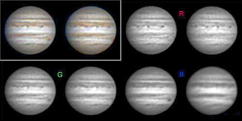
Although these two Jupiter images were obtained with the ST-6 just 30 min apart, planet rotation is already quite obvious (for instance, the Great Red Spot is already at the planet's limb in the second image). In consequence, the R- G- and B-filtered components of a true-color image of a fast-rotating planet must be obtained as quickly as possible. And each component is the average of various original images. Please notice the deterioration of seeing conditions at the time the last image was obtained. The most evident blur occurred in the blue-light image, which can be correlated to the fact that it had the longest integration time.

The final ST-6 RGB image of Saturn shown at the right was improved from its original counterpart (shown at the left) using the quadcolor L-RGB method described by Kunihiko Okano. In short, a higher definition grayscale image (in the middle) was used to replace the luminance channel of the original RGB image shown at the left. Although this grayscale and the original RGB image were obtained in sequence, the integration times were quite different (2 sec and 0.5 sec, respectively for filtered components and grayscale image), which explains the better definition of the former. Okano refers that the L-RGB method is very effective for planets. Further details of this method are presented at his web-site (http://www.asahi-net.or.jp/~rt6k-okn)
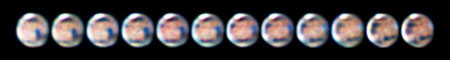
RGB sequence of planet Mars, obtained with the ST-6, demonstrating planet rotation. Polar cap, clouds, and albedo features like Syrtis Major can be recognized. Each RGB image was produced by merging three different grayscale frames sequentially obtained with color filters (red, green and blue). Sequences like this can also be used to produce time-lapse animations.
Image sequences thus obtained are good "static" representations of planet and satellite motion, but they can be readily used to originate time-lapse animations. I usually import the various TIFF files of a sequence, maintaining its relative position, into Microsoft VidEdit, which automatically combines all frames to produce a RGB or a grayscale AVI movie.
Time-lapse sequences of moving celestial bodies like those described above also allow us to recover three-dimensional (3D) information from the object that was imaged. In fact, a 3D-effect can be easily obtained by combining a set of two images acquired from the same site, with the same instrument and covering similar fields-of-view, but taken at a particular time-lapse from each other. This method can also be applied to solar system bodies other than planets. In fact, during a given time-lapse a rotating planet will show us a slightly different hemisphere, and a potential asteroid or comet will move with respect to the background star-field. Such images can thus be used to produce time-lapse emulated stereoscopic-pairs.
Time-lapse emulated stereoscopic-pairs of planets Mars, Jupiter and Saturn, all obtained with the ST-6. Both grayscale and RGB examples are shown. The left- and right-eye components are simply aligned side-by-side in order to be observed by voluntarily modifying eye-convergence (parallel viewing). Please try to look "through" the images so that left-right merging is achieved more rapidly.
Time-lapse emulated stereoscopic-pairs can be easily prepared using the red-blue color-coding or the side-by-side alignment methods. In the former method, a RGB image is synthesized by ascribing a previously obtained set of grayscale images, the future left- and right-side images, to the red- and blue-channel respectively. The image for the blue-channel is also used for the green-channel. The result is a grayscale anaglyph image. This can be readily achieved with image-processing software like Adobe PhotoShop. Such stereoscopic-pairs are then observed with colored 3D-glasses like those provided with one of the past issues of Sky&Telescope. They are made up of red and blue cellophane filters for the left and right eyes, respectively. In the latter method we simply align, side-by-side, a set of left- and right-side images that are then observed by voluntarily modifying eye-convergence (parallel viewing) or with the help of a binocular stereoscopic-viewer.
Grayscale anaglyphs of planet Jupiter (to obtain a 3-D effect please red-blue 3D-glasses) obtained with the ST-5C using image samplings of 0.8 (four images at the top) and 0.4 arcsec/pixel (bottom image showing satellites and satellite shadow). All images were obtained under favorable seeing conditions. The contrast of cloud features on heavily under-sampled images (0.8 arcsec/pixel) is high, although some spatial information is lost.
For both methods, choosing an adequate image size and obtaining a proper alignment of the resulting stereoscopic-pair are critical steps to obtain a correct 3D-perception. First of all, both images should have the same size and orientation. In order to maximize the 3D-effect, the object's path should be set horizontally, if necessary by rotating both images but preferentially by correctly orientating the camera before images are obtained. The rotation axis of planets should thus be set vertically. Image framing is also important. For rotating planets it is best to maintain a precise alignment of the planetary limb. An error that commonly occurs during the preparation of stereoscopic-pairs is the assignment of the left-side image to the right-side position and vice versa. Planets will appear hollow and with a concave surface. The optimum time-lapse between left- and right-side images depends of various factors, namely image magnification and speed of planetary rotation, and always has to be tested. If an insufficient time-lapse is chosen the 3D-effect will be minimum, whereas image merging will become difficult if an excessive value is used. An additional artifact appears when we chose a higher than desired time-lapse between images, namely a reduction of the planet's equatorial diameter. Satellite shadows can also be seen "floating" over the planet's surface when time-lapse emulated stereoscopic-pairs are used, which is an obvious artifact of the method.
Considering this background information, the next step in our perpetual quest to grab reality will surely be to attempt to produce 3D-animations from time-lapse emulated stereoscopic-pairs. And that is just a small step. I like to call the procedure that allows the preparation of 3D-animations the time-lapse parallax method. For spinning planets it is perhaps better described as rotational-parallax method, but it can be readily applied to other moving solar system objects. It completely relies in a single time-lapse sequence of images to originate the motion effect and to emulate parallax. The actual procedure is straightforward since all that is required is a 2D time-lapse sequence and some additional image-processing steps. In other words, previous 2D-animations can be reprocessed to obtain a 3D-effect.
To obtain a 3D-animation using the time-lapse parallax method I only have to shift two copies of same 2D time-lapse sequence by a given number of frames. For example, frame no.1 will become aligned with frame no.3, frame no.2 with frame no.4, frame no.3 with frame no.5, and so on. I then combine the newly aligned 2D-frames to obtain a sequence of time-lapse emulated stereoscopic-pairs. These stereoscopic-pairs are the actual frames I will use to build up the 3D-animation. Any of the two methods already described, i.e. the red-blue color-coding and the side-by-side alignment, is suitable to prepare such stereoscopic-pairs.
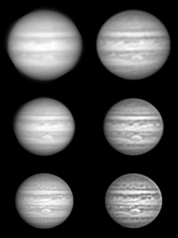
Grayscale images of planet Jupiter, imaged with the ST-5C under progressively more favorable seeing conditions (from top to bottom). All images on the left column were obtained at the same image sampling (0.4arcsec/pixel), and different sizes only reflect the planet's apparent diameter at the time the images were obtained. The images on the right column were obtained from exactly the same originals that produced the corresponding left image. However, each original was reduced 2x in size, prior to the same image processing steps referred in the text, in order to emulate an image sampling of 0.8 arcsec/pixel. This allowed a direct comparison of the effect of slight (left column) versus heavy under-sampling (right column) on image quality under different seeing conditions. It is evident that the images on the right are all more contrasted than those on the left, which can be highly advantageous to demonstrate subtle surface markings. Furthermore, only under the best seeing conditions (bottom images) there is an evident loss of information due to heavy under-sampling. This is because in all the other situations the theoretical resolution of the telescope could not be reached due to bad seeing. From my point of view, the most informative images under poor seeing conditions are those obtained at an image sampling of 0.8 arcsec/pixel.
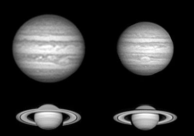
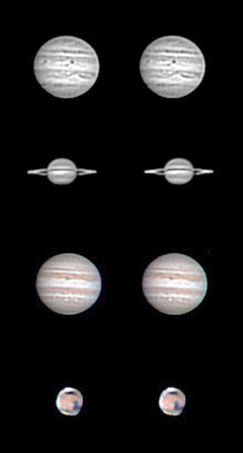
Grayscale images of planets Jupiter and Saturn obtained with the ST-5C at an image sampling of 0.4 arcsec/pixel under favorable seeing conditions. Numerous cloud features are identified on the planetary disks (e.g. the Great Red Spot and feestoons on Jupiter, and equatorial bands on Saturn). Small structures like the Encke minimum on Saturn ring system are also visible. The Cassini division is quite evident on both Saturn images.

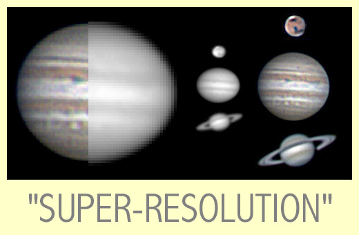
Grayscale images of planet Saturn obtained with the ST-5C at an image sampling of 0.4 arcsec/pixel under favorable seeing conditions. In those rare nights of very good seeing conditions, an image sampling of 0.4 arcsec/pixel (original sampling) may be insufficient to capture all the planetary details that are provided by the 10" telescope I use, unless if a "super-resolution" processing is applied. Much better results are in fact obtained when original images are enlarged (2x sampling) prior to averaging, an approach that produces a "super-resolution" effect in the final image. On the Saturn example shown above, the original sampled image (average of co-registered non enlarged originals) only shows the Encke minimum at the middle of the A ring. In contrast, the image subjected to the "super-resolution" method (2x sampling, i.e. average of co-registered enlarged originals) allows the visualization of both Encke minimum (at 50-60% out in the A ring) and the Encke Gap (very thin, located at about 80% out in the A ring). Some "on purpose" exagerated unsharp-masked sections of the rings from the original (2) and 2x enlarged final images (6), as well as from some original raw images of the original (1) and 2x sampling processings (3, 4 and 5) are also shown.
Well, I hope to have convinced you that obtaining a nice planetary image is not difficult at all, and that I have encouraged you to give it a try. In fact, what's difficult is to have constant access to a steady atmosphere, not imaging planets. In those brief moments where seeing is optimal do not hesitate and follow the Nyquist sampling criterion whenever possible. I'm sure you'll get the best possible results. When that is not possible for technical reasons, and on all the other less favorable nights, please don't give up! Go straight for the under-sampling approach and I’m sure you will "over"-surprised. Finally, and in all cases, remember that the results will much better if a series of (10-30) rapidly obtained planetary images are co-registered and averaged to get a final image. A single image will never be good enough after image-processing. So, want to snap a planet's portrait tonight?
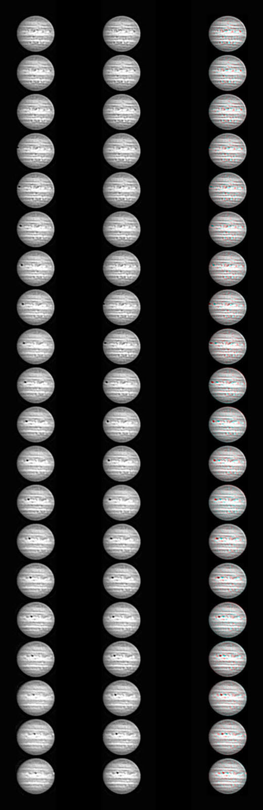
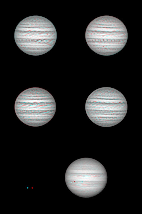
Sequence of grayscale time-lapse emulated stereoscopic-pairs of planet Jupiter, obtained with the ST-6. Satellite transit and shadow are evident. Two versions of the same sequence are presented: side-by-side alignment at the left (parallel viewing) and a grayscale anaglyph at the right (please red-blue 3D-glasses). Sequences like these can also be used to produce 3D-animations.
All Images and Texts on these pages are Copyrighted.
It is strictly forbidden to use them (namely for inclusion in other web pages) without the written authorization of the author
© A.Cidadão (1999)