REDUC TUTORIAL (V5.34)
|
REDUC TUTORIAL (V5.34) |
|
Load frames Reduc reads the following image formats: |
|
 |
Opens the classical Windows dialog box. The number of files that can be loaded is limited by Windows and it might be an issue with the huge number of images needed for speckle interferometry imaging or lucky imaging (read below Load Folder) |
 |
Load Folder is an easy to use and powerful loading routine. It enables to load a virtually unlimited number of files (>100 000, surely enough!). When the open dialog box is opened, select only one file and every file sharing the same extension in the folder will be loaded. It assumes that you recorded logically the frames of the observed stars into independant folders. |
 |
Modern softwares allow recording to FITS cube. This features loads and immediately expands a FITS cube. |
 |
Converts an AVI file into single BMP files. Proceed as follows to convert AVI files: |
Save files Reduc is able to write the following formats: Use the commands from : |
 |
| Main Window Most of the work is done on this window, so take a minute to localize some items |
1 Title bar displays the current frame's name |
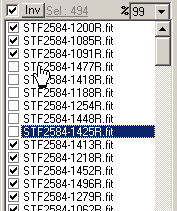
Files selection |
 |
Sort |
 |
Crop and Align This group of commands does what it says. It remains there more for educational purpose, when you will be familiar with Reduc you will use it very rarely. Double stars observers often take images of the small ROI (Region Of Interest) surrounding the double star to be measured. Align (...) reframes the images. At the difference of the simple crop the cropped area is defined relatively to the brigthest component found on the image. The effects of the adjustements are materialized by the red/white dotted cross. |
  |
Stacks Stack 10%...100% : sums the selected images. step 10%: sum of the first decile
These operations reframe the images. At the difference of the simple crop the cropped area is defined relatively to the brigthest component found on the image. The effects of the adjustements are materialized by the red/white dotted cross.
|
|
| Measurement overview | |
Two clicks for a centroid and four clicks for a measure: |
  |
Many things happen with these two clicks. Before all let's familiarize with the upper band containing the centroid detection settings. - The Section Area shows a section view of the star. The colors match the two axis colors of the zoom window. Maxi, Mean, Mini are the maximum, average and minimum pixels values inside the detection box. Current is the level value from which pixels are considered as significant for Reduc's centroid algorithms. This value is depicted by an horizontal dotted line which can be dragged to change the threshold. Moving this line forces Reduc to re-model the star and reestimate the centroid. |
 Note :  |
Reduction window |
|
The first right click on a star opened a window named Reduction. |
  |
| The first tab (Raw) activates the sheet of raw data. The three first columns are the coordinates and intensity of the main component, the three next contains the coordinates and intensity of the secondary component. The seventh column contains the name of the frame. The second tab (Reduced) activates the sheet of reduced data. Here are individual reductions of each frame with theta, rho, estimated mag difference and theta and rho residuals (individual measurement minus mean). In both sheets a click on a row recalls the corresponding frame in the main window. |
 |
| A color coding gives some informations about the measurements dispersion in the second sheet : Green residuals <= 0.674 s Blue residuals are >=0.674 s and < 2 s Fuchsia >= 2 s Take a look at right. Obviously, the last frame has a (hmmm) problem with a theta residual far greater than others frames in the set. Maybe a very bad frame, maybe an awkward click when measuring, who knows ? Click on the row, you can now suppress this measurement with the 'Delete' option on right click. When selecting the row, the frame has been recalled in the main window, you can now re-measure it if you want. |
 |
| Automatic Rejection You can discard an image having not enough quality. It's useful when you reduce a great number of frames. In the Reduction Window select Sort>Rejection. The analysis is instantaneous and the reduction lines are suppressed from the reduction tabs. The following criterions are used :
|
| Calibration Before reducing we need some informations : - Quadrants orientation: says if the quadrants succession is clockwise or counterclockwise - Relative pixel size (l x h): says if the scale if the same along x and y axis. Is generally the case but some imaging systems delivers frames with a different scale along the axes. Read about pixel size - Precise image orientation - Sampling (number of arcsec/pixel) |
From a calibration star : HOW TO PROVIDE CALIBRATION PARAMETERS |
Calibration with a calibration star It is the same procedure than a simple reduction. When the reduction is completed : Don't forget to switch to Measure mode before measuring ! NOTE : The second reduction sheet (Reduced tab) can't be displayed when in Calibration mode |
|
|
 |
Others calibrations |
Manual measurements After the calibration the precise image orientation and the pixel sampling are known. So you can switch to Measurement mode. Remember to press Clear before reducing a new target.
|
|
Publication and Information Logs
|
Advanced features
As an advanced double stars observer you already know that taking many frames of the target is the best way to ensure an easier reduction.
Reducing manually a great number of frames is not very funny, Reduc can make it easier and it is one of the nice parts of the use of the software.
In the advanced features you will find
- several methods to help to reduce a huge number of frames in the spatial domain: AutoReduc and ELI.
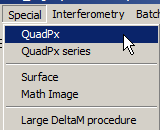
- the powerful Surface algorithm allowing the measurement of very close binaries and the helpful function QuadPx.
- a group of commands dedicated to Speckle Interferometry.
- two methods allowing theta calibration either on star trails or a set or of drifted frames.
- how to apply dark and bias preprocessing on the fly
- how to run several commands in batch mode
AutoReduc: Automated Reductions This method does the reduction of a set of frames automatically. It mimics a manual measurement on each frame, it reduces the frames independently. Select a good frame in the file list (BestOf might help) |
|
- Using the same way, select the secondary component and adjust if necessary the size of the search box. - Then click on 'comp B' |
  |
- And voila ! After a while the set of frames is reduced Depending on the seeing and the difference of magnitude, the brightest component may change from one frame to the other. If strict match is unchecked, Reduc uses all selected frames and defines the right orientation when the rank of magnitudes is inverted. After the completion the Disp. window shows the spatial distribution of the B component. The black square is the size of one pixel. |
|
ELI: Easy Lucky Imaging The basic principle of lucky imaging is to take many very short exposure frames of the target with the hope that a significant number (several %) of frames will be at least very sharp, at best diffraction limited. After a severe sorting the combination of the sharpest images gives a near diffraction-limited image. |
|
The procedure is similar to AutoReduc. During the procedure, Reduc might seem to freeze if you use several thousands of frames. Do not panic, let it run ! |
     |
After the completion of ELI: |
  |
SURFACE : Adjustment of a tridimensionnal surface Surface runs at full power on images with a high signal to noise ratio. Therefore it is not usable in the automatic reductions. |
  |
This picture (1) is beyond the Reduc's capacities. The centers of the stars are separated by a merely four pixels and the secondary component does not present a peak. |
(1)  |
| We said that it is necessary to click the brightest pixel of the main star. Reduc is going to help us to find it quickly. Adjust the research box to draw a wide window first (the centering is switched to Automatic)(2a) |
(2a)  |
Then reduce it to a 3x3 dimension, Reduc goes itself on the brightest pixel of the main component (2b). |
(2b)  |
| Click on 'comp A' button to identify the component (3) | (3) |
| The secondary component does not show a peak, it is impossible to reproduce this operation on it. First check the Manual option while keeping the size of the box to 3x3. Then, looking at the shape of the stars, click on the center of the secondary star. (4) | (4)  |
| Click the 'comp B' button to identify the secondary component | (5) |
Most of the time Surface does the reduction and we will see that just after. Here Reduc returns an error message (6). Surface cannot compute the positions of the components. |
(6)  |
Here the stars are too 'small' to allow Surface to work. |
(7)  |
Our stars now are of reasonable size. |
Before After QuadPx 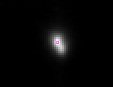 |
| This time Surface finds a solution to its equations. Our stars are measured. The numbers in the window are the calculated elements as Surface adjusts its equations: xA,yA,xB,yB,luminosity of A and B, the parameters of surface fitting , theta, separation in pixels and the gap between the mathematical surface and the picture. There is a line per iteration of the algorithm, generally greater this number, smaller the reliability of the measure. The program stops automatically when it reaches 25 iterations. Theta is computed with an internal orientation, it is automatically recomputed by Reduc according to the calibration of the orientation. |
(8)  |
| The results are sent to the Reduction sheet (9) | (9)  |
| The Surface's work can be verified by clicking on the measurement line.The big cross shows the center of A and the small cross the center of B (10). Don't be surprised if you see a light shift (1 or 2 pixels at most) between the crosses and the picture. It is a secondary effect when measuring the mathematical model. It is sometimes shifted to better calculation. Obviously a shift as the one of the picture (11) shows that something is wrong !!! |
 (10) Image measured correctly  (11) Someting is wrong !!! |
| Another quality of Surface is its stability. It can reduce correctly even though the component B is not perfectly identified. In case of doubt you can verify that the proposed solution is reproducible while changing slightly the position indicated for B. - Recall the picture by a click on the measurement line (12) - Click on a position slightly different of the center of B (13) and memorize its position (14). |
(12) (13)  (14) (14) |
| In this example we clicked voluntarily on a position very distant of the center calculated for B. However Surface provides a result equal to the later (15). | (15)  |
|
The Math Image option allows you to see how Surface has modelized the stars. - left the original image
|
(16) |
Resampling with QuadPx The command QuadPx Series does QuadPx on the Work buffer |
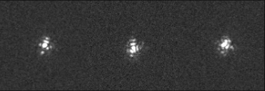
the original image, after a first QuadPx then after a second QuadPx |
Speckle Interferometry |
|
This chapter and the corresponding features of Reduc are dedicated to speckle interferometry technics. |
|
Autocorrelation Obtaining autocorrelogram with Reduc is extremely simple. Just click on Autocorrelation!
|
|
The algorithms use the fast Fourier transform (FFT). It requires square images whose dimensions are a power of 2. If your images do not follow this requirement, Reduc handles resizing before creating the autocorrelogram. Click OK on the error message and then choose a size compatible with your pictures in the next dialog box and then Ok Reduc then generates the autocorrelogram. |
|
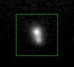
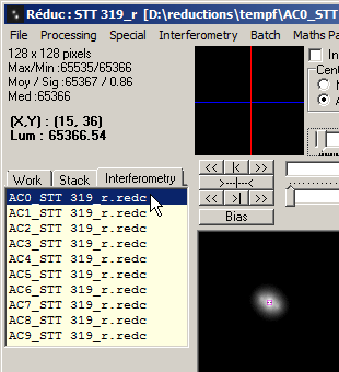
In the final computation, the file list shows the content of the interferometry buffer with 10 solution files named AC0_xxx to AC9_xxx. AC0 is the straight autocorrelogram. Autocorrelation peaks generally are embedded in noise and difficult to measure.
|
|
In order to highlight the peaks, the autocorrelogram is processed by a mean mask subtraction using a growing kernel (3x3, 5x5 ....). Files AC1 to AC9 are the result of this treatment. The problem is that the autocorrelation peaks are strictly symmetrical and there is always a 180° orientation ambiguity. To remove the ambiguity we can try to shift and add of several images or use the alternative offered by Reduc: cross-correlation
|
|
Cross-correlation The cross-correlation is another way to interpret the images of speckles. It has a main advantage because it allows to remove the ambiguity of 180 ° |
|
Transactions are strictly the same as for the autocorrelation described in the previous chapter. Load the images then click Cross-Correlation. Again the FFT is used and the warning about the dimensions of the images may appear => proceed as in the previous chapter.
|
|
In the final calculation, the file list shows the content of the interferometry folder with the 10 solutions (see previous section) |
|
It remains only to measure the peak corresponding to the secondary component. It is the brightest peak (*) (*) Actually the position of the secondary should be designed by the faintest peak. The internal process of Reduc reverse the image by 180° in order to show the secondary as the brightest peak. Just a question of easiness for the user :-) |
|
Images measurement The choice of the best solutions among the ten solutions computed must be adapted to your equipment and you'll have to test. However, here is a rule of thumb that can help to begin: Smaller the sampling, greater the number of the solution. Warning: |
|
The measurement is the same way that you measure a double star: |
|
Interferometry Fast Measurement Activating the Interferometry Fast Measurement option, we can now measure the correlogram with a single click.
|
|
A red message recalls that the function is active |
|
Select the peak to be measured and then right click Reduc computes immediatly the position angle and distance of the system and inserts them into the measurement window. Obviously the measured peak must match the B component Think of discarding the function if you measure later 'classic' images!
|
|
Do not hesitate to adjust the model window (yellow window) described above in the manual. By modifying the height of the horizontal line you modify the model and the number of pixels that are taken into account during the centroid computation. As far as the images permits, it is better to select heights giving a symmetric shape to the model as in the examples below. Reminder: a right click in the yellow window makes the measure |
|
 |
|
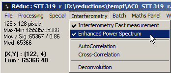
Enhanced Power Spectrum
|
|
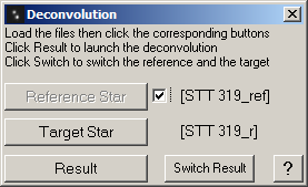
Deconvolution A common way to decrease the importance of the autocorrelation central peak is to divide the power spectrum of the target by the one of a nearby single star of same magnitude. The technique is powerful but quite complicated to implement properly during the acquisition of the images. Instructions for use: |
|
Star trail Calibration Three factors are important, the length of the trail, its time duration and the intrinsic quality of the picture. |
|
CALIBRATION : |
  (1)  (2)  (3) (3) |
| - Click a point at the other extremity of the trail. Again choose a place where the trace is well established (fig. 4) - Click now the 'B comp' button (fig. 5) |
(4)  (5) (5) |
|
(6)  (7)  (8) (8)  |
Synthetic Drift : drift calibration on multiple frames |
|
| - Load the set of frames, do not worry if they are not sorted - Adjust the size of the detection box so that it includes largely the star (fig. 1) |
(1)  |
| - Click on the 'Synthetic Drift' button (fig. 2) | (2) 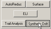 |
| - The pictures are displayed on the screen as Reduc analyses them. It is an opportunity to control that there are not any bad plots. - At the end the analysis a synthetic picture of the movement of the star is displayed and a dialog box asks for the orientation of the picture. It is time to give to Reduc the orientation of the quadrants. Click the corresponding button (fig.3) |
(3)  |
| - The calculated value are propagated automatically in the reduction sheet. (fig. 4) - The pre-orientation is put up to date too. (fig.5) |
(4) (5)  |
| If the curve of regression appears disjointed it is probably because there are incorrect frames. You can modify to leisure the selection of frames and you can launch again the analysis by clicking the 'Synthetic Drift' button. It's highly recommended to capture several drift series and to keep the mean value of their reductions as the final calibration value. |
|
Dark and Bias preprocessing Recall and basic principles:
|
|
| Preprocessing activation : 1/ Clic on the Bias button |
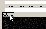 |
| 2/ Select the bias frames |  |
3/ Bias appears at the right of the button |
 |
| Stop preprocessing : 1/ Clic on the Bias button |
|
| 2/ Choose Cancel in the dialog box |
 |
3/ Preprocessing is stopped
|
 |
| Batch Procedures | |
The batch mode allows to run several commands automatically. The left board plays the following sequence of menu commands: The right board is dedicated to cubes pre-processing. It allows processing several cubes at a once. |
|
Maths Panel |
 |
Language I thank very much Edgardo Ruben Masa Martin, Gianpiero Locatelli and Antonio Adrigat for the spanish and italian translations. |
|
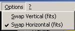
Horizontal and Vertical Swap
|
Cursors Set |
 |
| Visualisation levels The visualisation levels are computed automatically when Reduc loads a frame. Uncheck Auto to keep the same settings from one image to another. You can otherwise change them at any moment by moving the trackbars.
A false color visualisation can be obtained with the colored checkbox.  |
Logs Auto-Reload |
 |
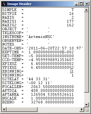
Image Header |
 |
Turbo Mode |
  |
| Customization of the camera list | |
Click on [...] button to customize the list. Delete a camera : blank all informations about it. ABOUT THE PIXEL SIZE |
|


 (17)
(17)