improving

After assembling colour CCD image as described before, the final result is often somewhat less than satisfactory. Usually low brightness/low contrast areas (for example outer arms of spiral galaxy) look quite noisy because of the uneven color. However, by transforming the original image into a "Lab" color space, one can re-process it to remove the effects of "color" noise.

While the approach based on the application of the separate luminance layer is already implemented in the so-called W-CMY and L-RGB color CCD images, here I describe an "extension" of that method. By creatively applying Lab model to already assembled images, it is possible to achieve more visually pleasing results. The improvement is the result of the differences in the "capacity" of various color models. Construction of L-RGB and W-CMY color images relies on the so called HSV color space (with capacity lower than RGB color model) to convert color and luminosity information - resulting image is then "extrapolated" into bigger RGB color space. Lab color model, on the other hand, can describe more colors than RGB space, so re-processing your luminosity and color data using that methods improves the final appearence of the color composite image. When its is converted into smaller RGB color space, it still looses some detail but the deterioration is very slight and the image looks a lot smoother.

"Lab" color model lets you split the image into completely independent brigthness (called luminosity or "L" layer) and color information (described as two independent chromaticity layers "a" and "b"). Each of those layers can be "manipulated" separately and they be combined back together into a modified color image.

Examples below demonstrate dramatic results possible with this method. It is important to remember that all the information was already present in your original FITS images. While color information in filtered images was most probably already uneven (due to lower signal-to-noise ratio), its distribution was further affected by data reduction into HSL color space. You still need good raw data to be able to see the improvement with Lab method.

This example shows the general application of Lab color space. All images were acquired with Cookbook 245 CCD camera on Celestron Ultima 8 f6.3 telescope autoguided with Cookbook 211 LDC CCD camera on piggybacked 500mm f8 telephoto lens. Eight unfiltered and -IR (white) filtered integrations (240 sec. each) were combined to creat white overlay (step 3). Five cyan, five magenta and six yellow exposures (240 sec. each) were combined into corresponding filtered images.

Steps 1 through 4 were done in AIP4WIN and all images were manipulated as 16-bit FITS files (their jpeg versions below had contrast enhanced so they display better on the monitor).

The output of step 4 was saved as 24-bit RGB tiff file and white layer from step 3 was also saved as 8-bit grayscale tiff.

Corel PhotoPaint 8 was used to convert and manipulate the above color and grayscale images in Lab color space in steps 5 through 8.

Final image was converted into 24-bit RGB tif and its compressed jpeg version is displayed in step 8 below.

Step 1. Calibrate and stack filtered images AIP4WIN was used for advanced calibration (bias, scaled dark and flat correction), subpixel registration, prescaling and averaging.

cyan-filtered image	magenta-filtered image	yellow-filtered image

Step 2. Convert CMY images into synthetic RGB layers. Solar analogue star-filter calibration data were used in AIP4WIN for this operation.

synthetic red image	synthetic green image	synthetic blue image

Step 3. Calibrate, stack and process unfiltered (white) overlay image AIP4WIN was used for advanced calibration (bias, scaled dark and flat correction), subpixel registration, prescaling and averaging. Resulting image was deconvoluted with Richardson-Lucy algorithm and then gamma-log scaled. Alternatively, filtered images may be added together to create a synthetic white overlay layer.

	white overlay

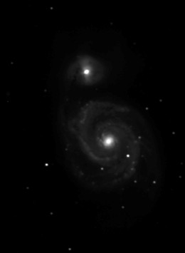
Step 4. Combine synthetic red, green and blue layers with white overlay AIP4WIN uses HSV color model to create color L-RGB image

	L-RGB image

What's wrong with this picture? bright areas (galactic nuclei) are burned out faint areas (outer arms) appear grainy due to uneven brightness and small scale color variations stars have uneven color What is going on here? the first two problems should be evident in white overlay (step 3) but that is not the case! uneven star color is caused by seeing changes during acquisition of filteres images and by small inaccuracies in image registration

Step 5. Convert L-RGB image into Lab color space and split it into individual layers Corel PhotoPaint 8was used to manipiulate color tiff image.


"L" layer (luminosity)	"a" layer (red-green balance)	"b" layer (blue-yellow balance)

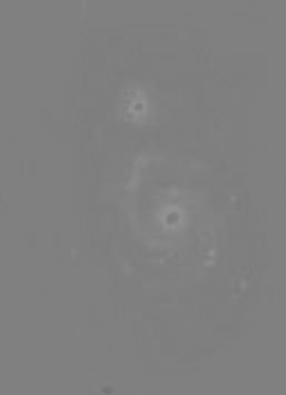
Compare L layer to original brightness information (white image from step 3) Luminosity information was clearly degraded during formation of L-RGB image. Interesting example is shown in the enlarged fragment of the image below - in this case a cosmic ray hit from a magenta-filtered image is visible as a dark spot in the luminosity information included in L-RGB image. It demonstrates that HSV-based approach allows cross-talk between color-filtered images (having lower signal-to-noise ratio) and a high quality white overlay, thus defeating the theoretical advantage of L-RGB (or L-CMY) method.


a part of magenta-filtered image with cosmic ray strike marked	the same region of white overlay image	corresponding region of "L" layer derived from L-RGB image

Step 6. To restore lost luminosity information, replace L layer with a white image from step 3 Step 7. To improve color definition of bright stars, apply gaussian blur filter to a and b layers from step 5


original white image = new "L" layer	blurred "a" layer	blurred "b" layer

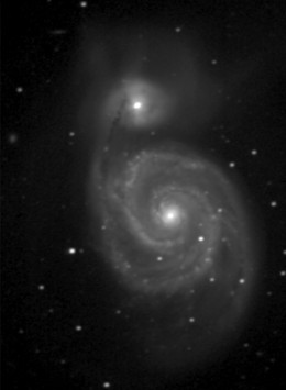
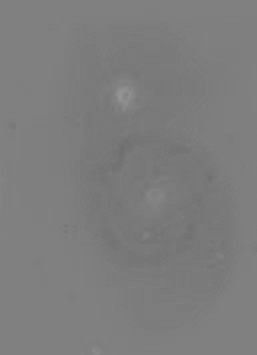
Step 8. Combine original white image and blurred a/b layers into Lab color image If needed, convert back to RGB, as Lab images cannot be compressed into jpeg format to published on internet.

Final Lab image (click here for full resolution version)	an enlarged fragment of Lab image corresponding to the area of cosmic ray strike in a magenta-filtered layer	the same area of L-RGB image prior to Lab processing

I hope this example speaks for itself ! Do not waste your precious photons to processing artifacts ;-)

Converting given color image into Lab color space and splitting it into component layers, allows unsharp masking of "L" layer only. When modified "L" layer is combined with "a" and "b" layers, resulting color image looks smoother.

Color images taken with short focal lenght optics (like telephoto lenses) suffer from unnaturally colored star images. Applying Gaussian blur filter to "a" and "b" layers significantly improves appearence of star images without affecting any nebulosity present in the same image.

The image below was taken with Cookbook 245 CCD camera an 135mm f4 telephoto lens.

Those are everywhere! Regardless of the target or integration time, there is always some faint outer arm of the galaxy or a barely noticable wisp of nebulosity present. In color images those areas get quite messy as there is not enough signal in CMY (or RGB)-filtered integrations. Human eye is quite sensitive to color variation. With "Lab" processing, however, that "noisy" color can be averaged to give low surface areas acceptable, though a bit washed out and sometimes greyish appearance. In this case, again, Gaussian blur (or even low pass filter) is applied to "a" and "b" layers. Sometimes all brighter stars loose color, but it is up to you to decide which component of the image is most important.

RGB images are formed from filtered-layers only. As such they sometimes suffer from low signal-to-noise ratios giving them grainy appearence. The easiest way to improve them is to add registered red, green and blue layers together to creat an artificial white image with better signal-to-noise characteristics. Then, it can be used in Lab color space as a new L layer with "a" and "b" data derived from the original RGB image (after conversion to Lab space as well).