|
HF
Propagation tutorial
|
|
|
ARCS
3D-modeling of the ionosphere. |
by
Bob Brown, NM7M, Ph.D. from U.C.Berkeley
Foreword
by Thierry Lombry,
LX4SKY (I)
Professor
Bob Brown, NM7M, worked as Physicist at University of California at
Berkeley, as expert of the upper atmosphere and the
geomagnetosphere. Until 2004, he was very interested in
propagation, and worked mainly on the top band of 160-meters.
Bob
Brown passed away on May 23, 2010. He was 87.
In
1998, Bob Brown wrote a syllabus about HF propagation for his students
that will become this tutorial in which Bob introduces us in the fascinating world of HF propagation.
It is at that time that I asked him the permission to publish his
syllabus on this site.
To
provide an accurate information to the reader, I took the freedom to
add illustrations and additional comments (referenced in
notes) as some information changed over the years (e.g. an URL); new
documents (studies, bulletin, models, images, etc) have been
released and are today available on the Internet as well as new
propagation prediction programs, as many information that, I hope,
will complete the already very useful information provided by the
author. These updates were made in 2004 and links as well as the
list of software were updated in 2014.
I
hope that this document will become one of your bedside book.
Ready?
Hop!, let's jump in the upper atmosphere in company with Bob.
Introduction
I
have to agree there is a lot of information out there on the
Internet; but what about understanding? Let me put out a few remarks
that might help your understanding of propagation.
First,
we depend on ionization of the upper atmosphere. That results from
solar ultraviolet, "soft X-rays", "hard
X-rays", and the influx of charged particles. Leaving the
charged particles out of the discussion today, the solar photons
have their origin largely in active regions on the sun.
Historically,
active regions were first counted and tallied, then the next step
was to measure their areas. Both methods have their problems with
weather conditions and after WW-II it was found that the
slowly-varying component of solar radio noise at 10.7 cm was
statistically correlated with the method using sunspot counts.
Later, with the Space Age, it was found possible to measure the
"hard X-ray" flux coming from the sun in the 1-8 Angstrom
range.
In
my opinion, the 1-8 Angstrom background X-ray flux is a better
measure of solar activity, at least for our radio purposes. Let me
explain.
First,
the X-ray flux has been found to come from regions more centrally
located on the visible hemisphere of the sun; that means a
significant fraction of their X-rays will reach our atmosphere.
Second, it takes 10 electron-Volts (eV) of energy to ionize any
constituent in the atmosphere; the energy of 1-8 A X-ray photons
exceeds that by over a factor of 100.
The
energy of 10.7 cm photons is .00001 eV, a factor of 1,000,000 too
LOW to ionize anything in our atmosphere. So the 10.7 cm flux only
tells us about the presence of active regions on the sun, not
directly about the state of ionization in the ionosphere. If that
was not bad enough, it has been found that the 10.7 cm flux can come
from the corona above regions which are behind the east and west
limbs of the sun. Those regions are much less likely to have their
ionizing radiation reach the ionosphere directly. So the 10.7 cm
flux has its purpose, indicating the presence of active regions, and
it is a mistake to think that changes in that flux are always
associated directly with the state of our ionosphere.
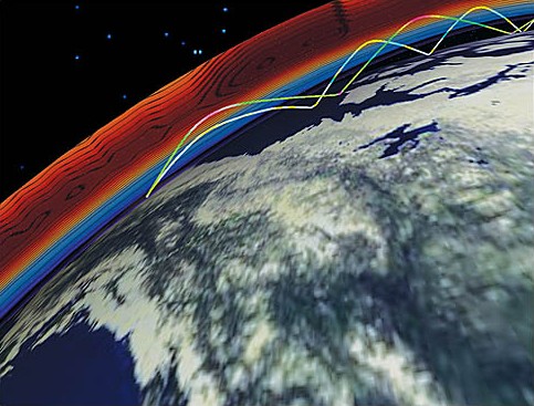
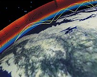
However,
as noted LX4SKY who provided the next plots, the solar flux at 10.7
cm is not without effects on the temperature and pressure of the
high atmosphere of the Earth as show well the documents display
below. This effect will mainly impact the lowest band propagation.
 |
 |
|
Correlation
between the solar flux at 10.7 cm and the variation of
the earth atmospheric pressure. At left the solar
cycle forcing (K per 100 units of 10.7 radio flux). On
the right image, at left correlations between the 10.7
cm solar flux (the 11-year solar cycle) and 30-hPa
heights in February, shaded for emphasis where the
correlations are above 0.5; upper panel: years in the
east phase of the QBO (the phase of the Quasi-Biennial
Oscillation determined using the wind between 50- and
40-hPa in January and February); lower panel: years in
the west phase of the QBO. At right, respectively,
height differences (geopot. m) between solar maxima
and minima (1958-2001). Documents Met
Office and K.Labitzke,
FUB. |
|
Having
said all that, let me conclude by pointing out the 1-8 A X-ray flux
values are given by NOAA in ranges which differ by a factors of 10,
such as A 2.3, B 4.0 or C 1.5. The numbers are the multipliers and
the letters give the category. Now I have logged the 1-8 A X-ray
flux through all of Cycle 22 and now into Cycle 23. The sum and
substance of my experience is quite simple: the A-range is found
around solar minimum, the B-range on the rising and falling parts of
a cycle and the C-range during the peak of a cycle.
So
what about Cycle 23
than will probably extend from 1997 to 2007? We suddenly moved out of the A-range (with
sporadic B-outbursts) in August of '97, hovered in the low B-range
until March '98, were in the mid-B range to the present time when
there were recent outbursts in the C-range. It is still too early to
say if solar activity has moved into the C- or solar maximum phase;
several months of data will be needed before any such estimate can
be made.
 |
 |
|
At
left the solar cycle 19 to 23 (from 1953-2005). At
right the solar flux at 10.7 cm from 1947 to 2001.
Documents SIDC and SPIDR. |
|
But
logging the 1-8 A X-ray flux, with 4-cycle log paper, will give you
insights as to the state of the ionosphere and recurrences in the
plot will serve to point out good/bad times for DXing. While spikes
in the 1-8 A diagram may suggest "hot times" for DXing,
they can be brief and difficult to take advantage of. It is more
productive to look at the broader peaks in flux in planning one's
DXing. The flares and coronal mass ejections associated with
outbursts of activity that take place now are more likely to give
bad propagation conditions because of all the geomagnetic activity
that follows. For DXing, the broad peaks are more productive.
All
of the above involved words, no great mathematical exercises. But I
like to tie it together mathematically using a simple proportion
that everyone can grasp quickly:
When
it comes to changes in the state of the ionosphere, X-rays are to
solar noise as, with DXing, beam antennas are to dipoles. OK?
Having
talked about the creation of ionization overhead, electrons and
positive ions, all sorts of practical questions come up at once. And some theoretical ones
too. We'll leave the theory to a later time, when DXing is slack
and there is more time to spare.
But
when it comes to practical matters, we have to throw our frequency
spectrum against the ionosphere and see how it all shakes out.
Of course, all that was done more than 50 years ago, one
frequency at a time, and the idea of critical frequencies emerged.
Those were for signals going vertically upward into the
various regions overhead, foE and foF2 for E- and F2-regions, and
gave the heights and frequency limits beyond which signals kept on
going into the next region or on to Infinity.
But
we communicate by sending signals obliquely toward the horizon and
that makes a difference, our higher frequencies penetrating more
than the lower ones before being returned toward ground. And we have to note our RF excites the electrons in the
ionosphere, jiggling them at the wave frequency, but they do collide
with nearby atoms and molecules, transferring some energy derived
from the waves to the atmosphere. That's how signals are absorbed, heating the atmosphere.
But
for electrons, there's a difference between being excited by 28 MHz
RF and 1.8 MHz RF. For
one thing, it depends on how often electrons bump into nearby atoms
and molecules. At those high frequencies, say 28 MHz, the wave frequency is
high compared to the collision frequency of electrons and absorption
losses are relatively small. The same cannot be said for 1.8 MHz signals on the 160 meter band and
the wave and collision frequencies are comparable, meaning that
electrons take up RF energy and promptly deliver it over to the
atmosphere.
One
can go through all the mathematics but you can almost guess the
answer: absorption is a limiting factor for the low bands, 160, 80
and 40 meters, and ionization or critical frequencies (MUFs) are the
limiting factors for the high bands, 15, 12 and 10 meters.
That makes the middle or transition bands, 30, 20 and 18
meters, ones where both absorption and ionization are important.
We
can phrase this in another practical way - 160 meter operators do
all their DXing in the dark of night when there's no solar UV or
X-rays to create all those electrons that absorb RF. By the same token,
the 10 meter crowd do their DXing in broad
daylight, when entire paths are illuminated, and they couldn't care
less.
Those
are the extremes but practicioneers on the "workhorse
band", 20 meters, have to put up with both uncertainties in
MUFs and the absorption by electrons. But in times like now, there is enough ionization up there to
support DXing at dawn and dusk, when the absorption is at a minimum.
For that band, Rudyard Kipling's ideas about "mad dogs
and Englishmen go out in the noon day sun" would seem to apply.
OK?
|

|
|
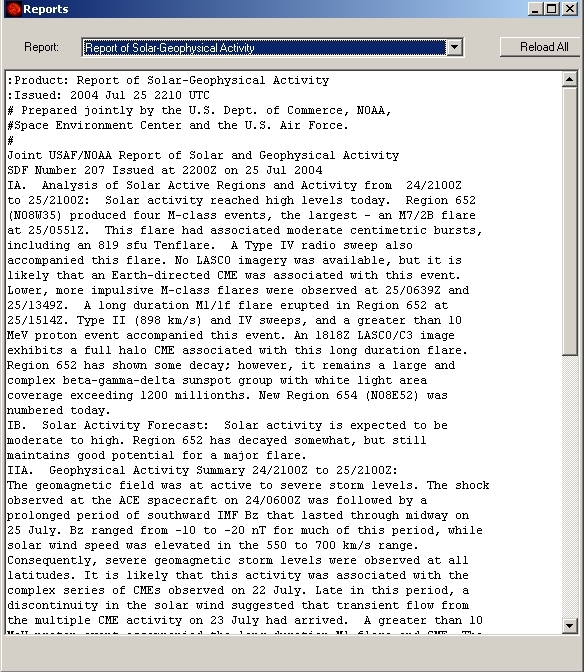
A
typical spaceweather report available online via the "DX
ToolBox"
software. |
Those
ideas, darkness and sunlight on paths, bring up the matter of
computing with mapping programs for checking darkness on 160 meter
paths and daylight on 10 meter paths as well as MUF programs for
bands from 10 MHz upward.
But
those last programs should also have a capability of giving
signal/noise ratios for the bandwidths appropriate for the modes. After all, getting a signal from a DX location is not worth
much if it cannot be read above the noise. For me, VOACAP
is at the top of the list but it has offspring and there are other programs that
can fill the bill. But I cannot stress mapping programs enough; you just have to see where
you're trying to go and the obstacles along the way, like the
auroral zones.
But
to use a MUF program, a measure of the current solar activity is
needed and effective sunspot numbers (Effective SSN) were for a
while available in "HF Prop"
bulletins from the Air Force and the Space Environment Center of
NOAA (SEC). Those numbers
were derived from observations of actual
propagation and amount to "pseudo-sunspot numbers". They
were more to the point than using
daily values of the 10.7 cm solar flux. However today only Part IV
of this bulletin is still available via the Internet. Other products
like IonoProbe from
VE3NEA also provides the Effective SSN and other real-time solar
data.
Note
by LX4SKY. The U.S.
Air Force no longer produces the "HF Prop" Bulletin.
They stopped this some years ago. However, the data in section
Part IV of the old bulletin can be found on SEC website at a
couple places.
For
example, under ONLINE
DATA click on "Near
Earth". "Near Earth Alerts and Forecasts"
have the daily Solar and Geophysical Activity Report and 3-day
Forecast. This product contains the Observed/Forecast 10.7 cm
flux and K/Ap.
Under
the "Near-Earth Reports and Summaries", the Solar
and Geophysical Activity Summary contains the Satellite
Background and Sunspot Number (SSN) in section E and daily
Indices (real-time preliminary/estimated values).
Today
VOACAP is available
online. At
last, recall that in a propagation program like DX
ToolBox, some of these reports can be read from within the application
(if you have an active connection to Internet of course).
Next
chapter
Effects
of the ionization
|