|
HF Propagation tutorial
|

|
|
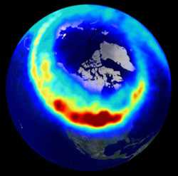
Composite
image of an aurora yielding a power of several GW recorded
in the visible and UV part of the spectrum by the Polar
satellite. |
by
Bob Brown, NM7M, Ph.D. from U.C.Berkeley
Effects
of the ionization (II)
Right
now, there's more than enough ionization up there to support DXing
on the low bands, 160 to 40 meters. But the higher bands are still pretty spotty, mainly across
low latitudes or in brief bursts of solar activity. But 10 meters will return; trust me.
The
discussion so far has dealt with the creation of ionization and how
various frequencies in our spectrum make out as far as propagation
and absorption are concerned. There's
one problem with that discussion, the omission of how, in the course
of time, ionization reaches the steady-state electron densities
overhead.
So
let's turn to that but do it as simply as possible. That means we'll focus on electrons, positive and negative
ions. The solar UV and X-rays create those from the oxygen and nitrogen molecules in our
atmosphere. I can say it is a big, complicated ion-chemistry lab up there
but we'll stay at the generic level, nothing fancy, just electrons
and positive ions.
In
simple terms, there is a competition between the production and loss
of ionization, just like your bank balance where depositing
paychecks and paying bills are in competition. So for us, there's a certain number of electrons created per
second in a cubic meter of air in the ionosphere by the solar
radiation and whatever the number of electrons present, some are
being lost by recombining with positive ions to form neutral atoms
or molecules again. If the two, gain and loss, are equal, there is a steady-state of
ionization; otherwise, there will be a net gain or loss per second
from some cause or other.
I
haven't said so but the atmosphere is only lightly ionized, say one
electron or positive ion per million neutral particles. So electrons have a greater chance to bump into a neutral
particle (like in ionospheric absorption) than a positive ion, to
recombine to make a neutral atom or molecule. And, of course, there's a vast difference in those rates
between the lower parts of the ionosphere, the D-region below 90 km
and the F2-region above 300 km. So electrons created by solar UV would be gobbled up rapidly
in the D-region but linger on for the better part of a day up in the
F2-region.
|
|
|
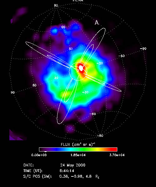
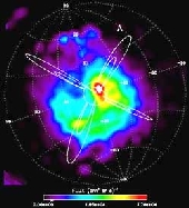
Solar
particles (protons and neutral atoms) hitting head on the
upper atmosphere of the earth over the equatorial region.
Doc NASA-GSFC. |
Good
illustrations of the fast processes are found nowadays, solar flares
illuminating half the earth with hard X-rays (like those in the 1-8
Angstrom range). They
penetrate to the D-region, release electrons which rapidly transfer
wave energy to the atmosphere. As soon as a flare ends, the sudden
ionospheric disturbance (SID) or radio black-out ends as the
electrons in the D-region recombine rapidly and signal strengths
return to normal.
The
lingering on of electrons in the F2-region is responsible, in part,
for the fact that there's still ionization and propagation in hours
of darkness. In short,
electrons at high altitude recombine slowly after the sun sets. But there's more to the story than that, the role of the
earth's magnetic field. Let
me explain.
The
earth's atmosphere is immersed in the geomagnetic field so any
charged particles, say ionization created by solar UV, will then
experience a force from their motion in the field. For electrons, that means they will spiral around the field
lines when released by UV and not fly off in any direction to
another location, higher or lower in the ionosphere. In the propagation business, that is called geomagnetic
control, meaning that the earth's field largely determines the
distribution of electrons in the ionosphere.
True, the solar UV creates them and they are most numerous
where the sun is overhead but they are held on field lines and
linger on after dark, to our great advantage.
But
the earth's field also creates problems, especially for the low-band
operator. It turns out
the gyro-frequency of electrons around field lines is about 1 MHz
and comparable to frequencies in the 160 meter band. Thus, a more general approach has to be made in the theory of
propagation at that frequency, adding the effects of the earth's
field on ionospheric electrons. The results are quite complicated, with
elliptically-polarized waves on low frequencies where
linearly-polarized waves were the story earlier on high frequencies.
That is a subject in itself and has to be left for a rainy day. But those are not
the only ways that the earth's field enters into the propagation
picture. Stay tuned.
Earlier,
I said there were other ways that the earth's field enters into the
propagation picture. But
that's sort of getting ahead of my development so let's backtrack a
bit and look at the historical picture.
The
study of geomagnetism goes back more than 100 years, well before the
advent of radio. It was
known that the occurrence of magnetic storms was related to the
solar cycle and, by the same token, it wasn't long before it was
realized that HF propagation was related to it too. The two really came together about 70 years ago when
commercial radiotelephone service was established across the
Atlantic Ocean. Then it soon became apparent that there were disruptions in service during
magnetic storms. You can find all that discussed in the I.R.E. journals in the early '30s.
In
that period it was thought that the ionosphere was the result of
solar UV, the photons reaching the earth 500 seconds (~8 minutes) after leaving
the sun. And while
magnetic storms were known to disrupt radio propagation, there was
no obvious connection as experience showed magnetic storms occurred
a couple days after the flash phase of a large flare on the sun. True, there was the idea of solar material, electrons and
protons called "plasma", approaching the earth after a
solar outburst and engulfing the geomagnetic field, even compressing
it. But the two effects
from plasma and UV seemed separable just because of differences in
time-of-flight across "empty space" that were associated
with the two effects.
But
all that changed with the Space Age when it was found that solar
plasma was out there all the time, the solar wind, and that it blew
past us with differents speeds, 200-1,200 km/sec, as well as
different particle densities and even carried magnetic fields along.
But for us earth-bound souls, the big surprise was that the
solar plasma distorted the earth's magnetic field, essentially
taking some field lines on the sunward side and pulling them back
behind the earth to form a magnetotail. Moreover, with the solar plasma coming at us, it became clear
that a ordered, dipole field did not go on forever, only out to 8-12
earth-radii in the sunward direction and even that depended on solar
activity.
So
what does this have to do with propagation, you ask. Well remember I said geomagnetic control of the ionosphere
means that electrons are held on magnetic field lines, making the
earth's field something of a reservoir for ionospheric electrons. But if field lines can be distorted, that would surely affect
the density of ionospheric electrons gyrating around them and
propagation.
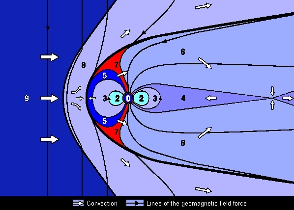
The
worst-case scenario is when field lines are dragged way back into
the magneto-tail by an increase in solar wind pressure, taking
ionospheric electrons with them. That field configuration is sketched crudely below where two
compressed field lines are shown in front of the earth, in the solar
direction, and two magnetotail field lines in the anti-solar
direction as displayed below.
|
Structure
of the geomagnetosphere
|
|

|
0
- Earth
1
- Ionosphère encircling the Earth (not shown)
2
- Plasma sphere
3
- Van Allen belts
4
- Plasma sheet (internal magnetosphere)
5
- Magnetopause
6
- Geomagnetic tail
7
- Polar cone
8
- Geomagnetopause
9
- Solar wind
Clic
on image to enlarge. Document BAS.
|
|
That
would mean a depletion of electrons at F2-region heights and drastic
reductions in MUFs, affecting propagation. Fortunately, that fate is reserved
primarily for sites at high latitudes, around the auroral zones and poleward.
What
I described was what takes place during a major geomagnetic storm. The recovery is a slow process as ionospheric electrons have
to be replaced in the usual way, by solar UV and day by day while
the sun is up. So it can take days for the bands to recover when a strong
magnetic storm reduces MUFs by a large fraction.
Now
to be practical again, magnetic activity on earth is caused by
interactions of the solar wind out there at the front of the
geomagnetic field. The
field region around the earth is called the magnetosphere so we're
talking about effects on high latitude field lines that go out to
the magnetopause, the dividing surface between terrestrial and
interplanetary regions. But it must be recognized that this sort of
thing is not toggled on and off; it is going on all the time as the
solar wind sweeps by. It is just a matter of
degree. But how to deal with it in DXing?
The
clue comes from an interaction within the magnetosphere, local
electrons being accelerated to high energies and then spiralling
down field lines to make visible aurora and ionization at E-region
heights. Those events are triggered by solar wind interactions at the magnetopause and
accompanied by horizontal currents in the E-region that show up in
magnetic observations on the ground. It then becomes a matter of using the
strength of the local magnetic effects at auroral latitudes, with K- and A-indices like
those you hear about on WWV or can check on DX
Summit Cluster (OH8X) or DXHeat, to judge the energy input from the
solar wind as displayed below.
To
read : The
Shape of the Sunspot Cycle (PDF), D.Hathaway
and al., NASA
 |
|
WWV
data provided by NOAA. |
|
To
bring this to a conclusion, good propagation conditions are found
when there is a strong UV input to the ionosphere and low magnetic
indices, the 3-hour K-index less than 4 and the daily A-index less
than 25. Dreadful
propagation conditions were found recently in the magnetic storm of
August 27 when K reached its limit, 9, and the planetary average of
the A-index was 112. But it could have been worse! However,
let's look at the brighter side next time, how signals get from A to
B.
Let's
leave a curved ionosphere to later and do some "Flat-Earth
Physics" to see how signals get from point A to point B. For that we start with a simple model of the ionosphere in
which the electron density increases upward and peaks at about 300
km altitude. That's something like a night-time ionosphere.
Now
it may seem strange but one can draw an analogy between the flight
of a baseball and RF going up through that ionosphere. For the baseball,
high school physics teaches you how to calculate how high a baseball
would go if thrown vertically upward. In college, the ball is thrown or hit upward at an
angle. The method is the same in both cases: the ball rises until
the increase in its potential energy in the earth's gravitational
field is equal to the kinetic energy it had from its initial
vertical motion.
Neglecting
friction, the baseball's path is a parabola that is symmetrical
about its highest point and the ball returns to the ground at the
same angle to the vertical as it was launched. While not really
parabolic in shape, the flight of RF through that simple ionosphere
is similar, reaching a peak altitude that is determined by the
frequency and launch angle, symmetrical about the peak and returning
to ground at the same angle. How does that happen? Let me explain.
The
flight of a baseball and the path of RF in a simple ionosphere are
determined by gradients, of the gravitational energy of the ball in
the first case and the electron density distribution in the second
one. There is a gradient of either of those quantities if there's
a change in value with altitude, say gravitational energy or
electron density greater at higher altitudes than lower at altitudes.
The gradients are responsible for the bending or curvature of
the paths in the both cases and, numerically, they are given by the
change in value per km change in altitude. OK?
In
spite of all the "Home Run Fury" these days, let's leave
the baseball part of the analogy and focus on what happens to RF.
So we see that hops, with RF rising and then returning to ground,
are the result of the vertical gradient of the electron density in
the ionosphere. On reflection at ground level, angles of incidence
and reflection are equal and the path continues upward again.
But
there can be horizontal gradients as well, say across the terminator
where there is more ionization on the sunlit side than the side in
darkness. So if RF
signals were sent initially parallel to the terminator, one would
expect the RF to be bent away from the sunlit side, with its higher
level of ionization, and toward the darkness. Right? That's
skewing, pure and simple, with the RF refracted away from the region
of greater ionization.
The
height a baseball reaches depends on its speed and direction; for
RF, that translates into frequency and launch angle. But one sees that from different
arguments. Let me add a few words there. At any height in the
ionosphere, there are electrons and positive ions. If, by mystical powers, you could grab a handful of each and
then pull them apart, they would be attracted to each other by the
electrical forces between unlike charges and on release, they'd
swish back and forth, carrying out an oscillatory motion. The
frequency of that motion is called the plasma frequency and it
depends on the density or number of particles per unit volume, N.
For
the ionosphere, where ionization increases with height, the plasma
frequency increases too. For
our night-time case, the peak electron density in the F-region might
correspond to a plasma or critical frequency of 7 MHz for the
F-region. Now vertical
ionospheric sounding shows that pulses of RF below 7 MHz would be
returned to ground while any above 7 MHz would penetrate the peak of
the ionosphere and go on to Infinity.
 |
 |
|
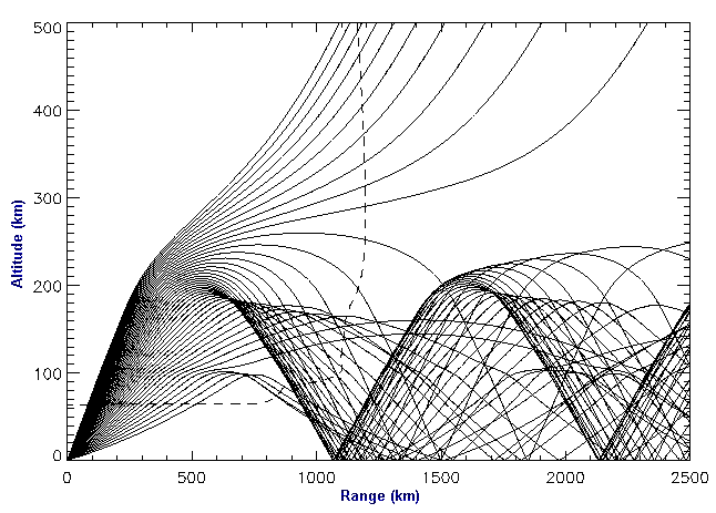
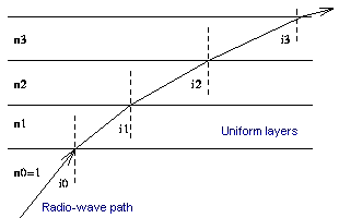
At
left, the refraction of a radio wave in a plane
stratified medium. Since the plasma frequency (critical
frequency) increases with height, n becomes smaller and
the wave gradually bends toward the horizontal. At right
a side-view of propagation paths of SuperDARN rays in
the ionosphere at a frequency of 12.45 MHz for elevation
angles from 5 to 50°. The dashed line indicates the
electron density profile. Documents realized by Andreas
Schiffler on a home computer using a ray tracing
program solving a set of differential equations. |
|
For
oblique propagation, we have to find the effective vertical
frequency of the RF, just like the vertical component of the
baseball's velocity. For
RF, it's found the same way, multiplying the frequency by the cosine
of the zenith angle at launch. So, in the "Flat Earth" approximation, 7 MHz RF
launched from ground at 30° above the horizon (or 60°
from the vertical) would have an effective vertical frequency of 3.5
MHz. OK, the
"baseball analogy" would say that the RF going off
obliquely would rise until it reached a height where the local
plasma frequency is 3.5 MHz and then return to ground. Of course, it would be on a curved path, the RF would be
moving parallel to the earth's surface at the top of the path and
returning to ground at the same angle as when launched, just like
the baseball problem.
In
baseball, there's friction and that changes the flight of a
baseball. We don't put "friction" in the RF problem. Instead, the electron density at a given height may vary
along the path direction, say become smaller. That would serve to "tilt" levels of the ionosphere
upward and weaken the density gradient. As a result, there would be less refraction or bending after
the peak altitude than before, and that tilt serves to increase the
length of a hop and change the RF angle on return to a lower value.
In
reality one would expect some change in electron density along any
path, increasing as a path goes into sunlit regions or decreasing
when going into the dark. So even if nothing else changed, one would not expect hop lengths nor
radiation angles to always remain exactly the same all along a path.
The
above approach, equivalent to mirror reflections of RF, is Newtonian
in the sense that the analogy treats a RF path like that of a
particle (baseball) and not a wave. When the Maxwellian or wave approach is carried out, one
finds that refraction is the same except that the effects vary
inversely with the square of the wave frequency. So in a given part of the ionosphere, 80 meter RF paths are
refracted or bent much more than 10 meter RF paths, either
vertically or horizontally. OK?
MUF
and RF attenuation
|
|
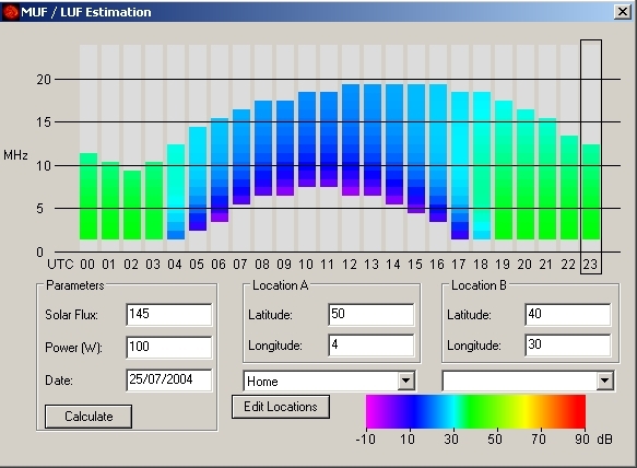
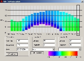
|
MUF/LUF
and signal strength estimation for July 25, 2004 calculated with DX
ToolBox for a power of 100W PEP from ON to TA. |
OK,
now we have the idea of critical frequencies and hops so it is no
big deal to work out how propagation on a path may be open or closed
for DXing on a given frequency. But to do that, we need at least map of where the RF is
headed and an idea of how many hops would be involved. Beyond that, some ionospheric details are required, the
critical frequencies along the path at the date and time in question.
If
one gets into the mathematics of all this, it turns out that hops
via the F-region may reach about 3,500 km and half that via the
lower E-region. So
using those ideas, one can estimate the hop situation, at least as
long as there is not a mixture of E- and F-hops. So consider a path
from my QTH in the Northwest to London, some 7,500 km in length.
That would work out, to a first approximation, to 3 F-hops of 2,500
km each.
Now what about the critical frequencies at the peaks of the
hops; how high are they and what bands might be open to me, say at
1200 UTC?
To
answer that question, one would need some sort of database, an array
of observations from which an estimate could be obtained by
interpolation, or a mathematic simulation of the database that could
be used to calculate the critical frequencies. Actually both methods are used in modern propagation
prediction programs but either way, appropriate numerical values
could be obtained for the peaks of the hops. But what to do with that data?
For
a one-hop path, the matter is simple; the effective vertical
frequency of the RF that is launched must be less than the critical
frequency for the path to be completed. No problem. For two hops, the effective vertical frequency of
the RF must be less than the SMALLEST of the critical frequencies of
the two hops to have a complete path.
And the operating frequency that gives the highest effective
vertical frequency that can complete the path is called the Maximum
Useable Frequency (MUF) for the path at that time and for the
corresponding solar conditions.
But
the path from my QTH to London involves 3 hops; what's the story
there? Historically, the idea was handled like the 2-hop path, using the critical
frequencies at the first and last hop to determine the MUF. The idea was that if propagation failed, it usually would be
due to conditions at one end of the path or the other. Anyway, this is called the "control point" method
and is used in most simple propagation programs. More sophisticated approaches would use critical frequencies
at each and every hop and the lowest would be the important one that
limits propagation.
 |
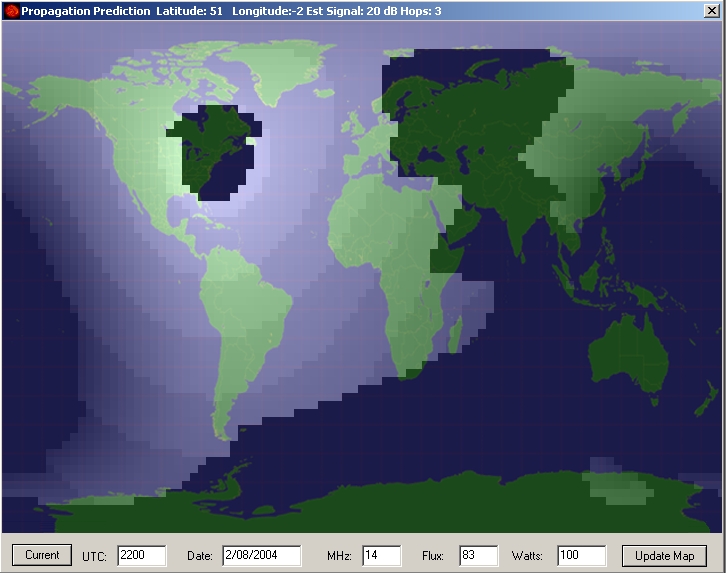
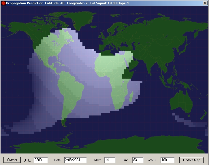
 |
|
Propagation
charts for the 20-m band on August 2, 2004 22:00 UTC for
paths from respectively New York to London and vice
versa. In both case of course the number of hops is 3 as
listed in the blue upper bar. The estimation map are
different because at that time the position of the Sun
is simply not the same over both QTH. Estimation calculated
with DX ToolBox by
LX4SKY. |
|
It
should be noted that the control point method would be quite
satisfactory for MUF calculations so long as the critical frequency
of the middle hop is not less than those at either end of the path.
That would be the case for paths going across the more robust
ionosphere at low latitudes where the sun is more overhead during a
day. But MUF
calculations using two control points for high latitude paths, like
from the Northwest to London, can be misleading as the critical
frequency for the middle hop (over Northern Canada and Greenland for
the path to G-land) could be lower than at the end points and thus
propagation not supported across the entire path using the MUF from
control points.
The
MUF calculations play an important part in propagation predictions
but it must be remembered that signal strength, in comparison with
noise, is an important consideration. As noted earlier, ionization and
MUFS are more important for the higher ends of the amateur spectrum and signal/noise
considerations for the lower end. In any event, for communication a path must be open or
available and signals must be readable and reliable.
All
of the discussion up to this point has dealt with propagation from a
conventional viewpoint - determined by the ionosphere that is
overhead and, in turn, one controlled by the level of solar activity.
Obviously, propagation is a complicated process and it may seem a bit naive but
we try to make all our predictions on a given date using using
databases which rest on only a few numbers - sunspot number and
magnetic indices. It is
not surprising that predictions are not 100% reliable. Such high expectations would deny the variability of the
original data input from ionospheric sounding and not reflect the
roles of dynamic solar variables.
So
far, this brief summary of the principal points that are involved in
HF propagation has been largely centered on words and concepts. More
advanced topics require a good deal of graphics so I will make appeal
from time to time to a figure or two in one or more of the reference
books given earlier. While figures are the best way to convey some of the material, I
will also try to put the ideas in simple words that will carry most of
the meaning.
To
me, the study of ionosphere and propagation changed markedly with
the advent of the Space Age. Thus,
with the International Geophysical Year (IGY) in '57, high-altitude
balloons, rockets and satellites began to probe the regions where
only radio waves had been before. So the "Photochemical Era", where solar photons and
atmospheric processes were thought to control the dynamics of the
ionosphere, gave way to the "Plasma and Fields Era" we're
in now, where the interaction of the solar wind with the earth's
field and the atmosphere are the controlling factors for
propagation.
In
simple terms, hams no longer look out the window for their local
weather, determined by the day, time and season, but now turn to the
Internet to get a daily report on the Space Weather. In a sense,
propagation and DXing just became less mysterious and even more
interesting. That's
what we'll be pointing toward in next pages, preparing for all the
details in last section.
It's
no secret that success in DXing means getting signals to and from a
DX station and also having them heard and read at both ends of the
path. But between those
two ends, a lot of things happen in the ionosphere and some of them
seem like well-kept secrets. So the hope is some of that can be
dispelled by the discussion which follows. But we need a beginning and the question is where to
start. Let's take the easy way and cover old ground first, the
matter of ionospheric absorption that was discussed in the second
session.
So
we go back to the idea that RF excites the electrons in going across
the ionosphere, jiggling them at the wave frequency. And they collide with nearby atoms and molecules,
transferring some energy derived from the waves to the atmosphere. That's how absorption takes place, mostly down in the
D-region. But there's a
frequency dependence we should talk about now, how absorption varies
with the operating QRG and with height, since the collision
frequency of the electrons is not constant; instead, it decreases
with height and that's a help. So it's clear now that ionospheric absorption is a little
more complicated than I first let on back in the introduction.
But
one can get a handle on it by looking at the extremes, low in the
D-region, say around 30 km where the collision frequency is greater
than any of the frequencies in our spectrum. In that circumstance, collisions happen so often the
electrons never have a chance to pick up any energy from the passing
RF.
On the other hand,
at high altitudes, say around 100 km, collisions are quite
infrequent and the electrons re-radiate most of the energy they
acquire and transfer very little to the atmosphere by collisions.
So
it is in between, where wave and collision frequencies are
comparable, that electrons take up RF energy efficiently and then
promptly deliver it over to the atmosphere. So with collision frequency falling with increasing altitude,
28 MHz RF is absorbed at lower altitudes than 3.5 MHz RF, as shown
at right. That graphic illustrates something that DXers know already, lower
frequency signals are absorbed more than higher ones but it shows
where it all happens. That's news, at least for some.
To
go beyond that qualitative result, one must have an analytical form
to represent the curves, call it F(f,h) for frequency f and height h.
Then multiply F(f,h) by the number N of electrons per cubic meter at height h and include
the physical constants to give the right units, dB/km. When all is said and done, the result is:
Attenuation
(dB/km) = 0.046 x N x F(f,h)
But
that is only at one place, where the electron density is N. Our
DXer's signal is attenuated by ALL the electrons encountered along
the RF path from point A to point B so that means we need to know
something about the propagation mode, the distribution of electrons
and add up the results, km by km along the path.
That's
a tall order but when it's done, it will enable our DXer to find
just how much of the radiated power P survived in going from A to B.
But whether our DXer can be heard still depends on how well
the attenuated signal compares with the noise power getting to the
receiver at B. But I'm getting ahead of myself.
|
|
|
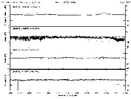
30
MHz riometer absorption. Document IPS. |
The
crude graphic shown at right can help in understanding a lot of simple
things. For example, it
is possible to identify various ionospheric disturbances just by the
absorption they produce. One
approach is to use an HF receiver to monitor the galactic radio
noise coming in vertically on 30 MHz. Galactic noise gets right through the F-region as 30 MHz is
above its critical frequency, even at equatorial latitudes where it
might reach 20 MHz in a solar cycle.
That instrument is called a riometer, for Relative
Ionospheric Opacity Meter, and they are generally deployed at high
latitudes where ionospheric disturbances are most common.
The graphs displayed at right for example have been recorded
over the Australian Antarctica base in 2004.
So
now, if some disturbance increases the electron density in the D- or
E-region, we see that the galactic noise signal will be attenuated
and indicate the presence of a disturbance.
But there are disturbances and then there are disturbances. So the graphic also tells us that anything that disturbs the
lower D-region will produce strong attenuation of the galactic radio
noise and, electron for electron, the attenuation will be much less
if the disturbance produces ionization at much higher altitudes.
The
first case would be for polar cap absorption (PCA) events, like we
all experienced in May of '98. In
those events, solar protons produce lots of ionization around 40-50
km altitude and give rise to tens of dB of additional absorption on
30 MHz and blackout oblique communication paths going across the
polar caps. Auroral events, say associated with magnetic storms,
give rise to strong ionization above 100 km, where the graphic shows
the absorption efficiency is much lower, and auroral absorption (AA)
events show only a few dB of absorption of galactic noise on 30 MHz.
Of course, there are other differences in the two types of
events, how the ionization is distributed in latitude and longitude
and how long they last. More on that later.
|

|
|
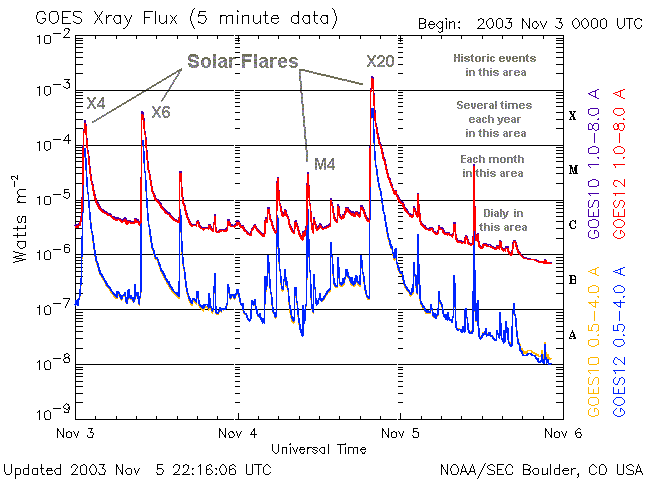
Severe solar X-ray flux recorded on November 4, 2003 by GOES satellites. Document SEC. |
One
last disturbance, again something that was within our recent
experience with all the flare activity in the summer of '98, is
sudden ionospheric disturbances (SID) from bursts of solar X-rays.
Those X-rays, in the 1-8 Angstrom range discussed earlier, were
incident on the sunlit hemisphere of the earth and literally swamped
the normal distribution of ionization at low altitudes, giving
intense absorption of signals going across the sunlit region. But experience shows, and the graphic indicates, that the
effects were worst at the lower ends of the spectrum, wiping out 75
meter operations but having little effect on 28 MHz, except perhaps
for some solar noise bursts associated with the flaring.
If
this would be quite academic, perhaps, were it not for the fact that
one can use the Internet to see these events in action or shortly
thereafter. Thus, records from the X-ray Flux Monitors on the GOES 10 and 12 satellites
are available at SEC/NOAA,
giving more meaning to the idea of an SID.
We'll
get to that later on but the main thing for us in the records is
that plots for 0 degrees tell what is going down into the
atmosphere, making more ionization and affecting the ionosphere.
The 90-degree plots involve particles trapped in radiation
belts and are more colorful than informative.
While
disturbances come and go, affecting our ability to work DX, we
really need to know something about the normal situation, say the
distribution of ionospheric electrons with height as well as
latitude and longitude. That
is a big order but, believe it or not, it can be contained in one
computer hard disk. I'm talking
about the International Reference Ionosphere (IRI),
the summary of decades of ionospheric sounding all over the world. So it will provide data on the robust part of the ionosphere
at low latitudes where the sun is more overhead and the
mid-latitudes where the ionosphere is more seasonal in its
properties.
But
the model is not reliable at high latitudes, say from below the
auroral zones and poleward. That
region is under the constant influence of the solar wind and
electron densities are highly variable, even hour by hour.
So that model has its limits.
But to bring the model to life, one needs a mapping program
to show the vertical and global distribution of ionization. Fortunately, we now have such a program available to
amateurs, the PropLab Pro program from
Spacew. I'll have more to say about that next time.
Reference
Notes
-
A better representation of the relative absorption efficiency per
electron as a function of height and frequency in the D-region is
found in Figure 8.1 in my book,
The
Little Pistol's Guide to HF Propagation.
-
And a more detailed
discussion of the analytical form, F(f,h), is found in Section 7.4
(Ionospheric Absorption) of Davies' book, Ionospheric
Radio (IEE Electromagnetic Waves Series, Vol. 31), beginning on p.
214. Also, the variation of collision frequency with height is
given in Figure 7.5 on p. 215.
Next
chapter
Distribution
of ionospheric electrons
|