|
HF Propagation tutorial
by Bob Brown, NM7M, Ph.D. from U.C.Berkeley
Geomagnetic
disturbances (VIII)
The end of the second volume of the book, "Geomagnetism"
by Chapman and Bartels, has an interesting account dealing with the
first days of magnetic observations in Sweden by Celsius and one of
his graduate students. Knowing what we do now, I consider that as
"Day One" of the Space Age. But I have to
marvel that it took 75 years until Oersted came up with the idea of
a current (like an ionospheric electrojet) giving rise to magnetic
deflections (on the ground below an aurora) of a compass. Compare
that time with the five years it took the French mathematicians to
come to grips with the Biot-Savart Law for magnetic effects of currents. Interesting!
Finally,
an excellent discussion of early auroral observations in Norway can
be found in the last chapter of Brekke's book, "Physics of the
Upper Polar Atmosphere" published by Wiley & Sons in
1997. Brekke, being a Norwegian, pays homage to the works and
tradition of good auroral physics established by Stoermer. It's
worth a bit of reading time, believe me.
At
the end of the previous page, we made note that magnetic storms give
rise to auroral disturbances, with optical emissions coming from
above the 100 km layer, VHF reflections off the ionization in
auroral displays, ionospheric absorption of signals going across an
active auroral zone and strong magnetic disturbances observed on the
ground from the current systems which develop along the ionized
region. All that from
an enhancement in the solar wind, perhaps coming at a greater speed,
with a greater particle density or with the interplanetary magnetic
field pointing south with respect to the earth's field.
Nowadays,
we can read about all those changes on the Internet. But the most
important one for magnetic storming has to do with the
interplanetary field and its orientation. With the field pointing south, conditions when Bz is
negative, the interplanetary field can merge with the terrestrial
field (a non-classical concept) and field lines on the front of the
magnetosphere then transferred to the tail region as the solar
plasma sweeps by.
These
ideas came forward in the '50s, thanks to the efforts of J. Dungey
of the U.K. and others. As I said earlier, they go beyond the elementary
considerations we get in classical courses on electromagnetic theory and
are best left for the theorists to discuss. We
only need to know what happens to the ionosphere and there, the news
is BAD as the F-region loses ionization with the development of a
magnetic storm.
But
the E-region can gain ionization, with the penetration of auroral
electrons. Those
particles are from here inside the magnetosphere itself, not
directly from the solar wind, and are accelerated locally, going
from a fraction of an electron-Volt up to tens of kilovolts energy.
And their flux can be quite large, resulting in electron
densities of a million or more per cc from electron collisions with
atmospheric constituents in the tens of kilometres above the 100 km
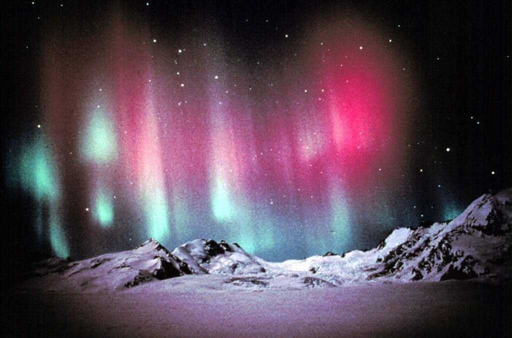
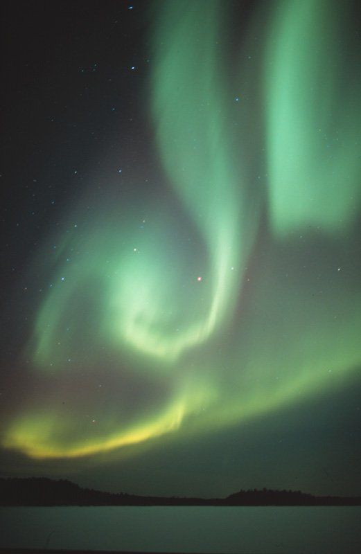
level. The colors of the aurora are testimony to the collisions with the neutral
constituents and the electron densities that result can give rise to
signal absorption.
That
last point may seem strange if you go back to the curves that were
given page 2. There, the relative absorption efficiency per electron was
dropping off quite rapidly above 100 km. But in the case of aurora, there are millions of electrons
per cc up there and even if electron-neutral collisions are less
frequent above 100 km, losses result just from the sheer amount of
ionization that goes with an aurora.
But
to give some numbers, auroral absorption of up to 5 dB or so is
found in the riometer records of 30 MHz galactic radio noise coming
in vertically. But that is just for one pass through the ionosphere.
For amateur communications, say on 28 MHz, that should be doubled for
a complete hop, increased even further by a factor of
3-4 for the oblique angle of the path and adjusted for the
inverse-square frequency variation. At lower frequencies, that last
adjustment shows even greater losses on those bands. So
it should be no real surprise that auroral absorption represents an
adverse factor for amateur communications.
|

|
|
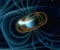
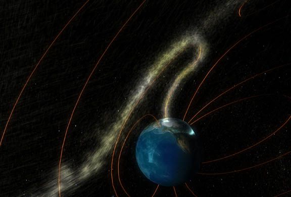
This
drawing illustrates an electromagnetic reconnexion (between
the solar wind in yellow and the geomagnetic field in red)
called a "crack" in the shield protecting earth.
This is through such cracks, as large as a state and
remaining open for hours, that the solar flux can
penetrate into the ionosphere and create auroral events. Click
here
to run the animation (1.7 MB MPEG file) prepared by NASA/GSFC. |
Those
remarks dealt with the electron density; one should also note the
geometry and activity of the aurora. In regard to geometry, auroral
activity at any given time is restricted to a narrow latitude range.
(See Research Notes) But it can extend over a wide range of longitude
and the type of activity varies from west to east. In evening hours,
aurora tend to be quiet and not involve a lot of energetic particles
(and ionization). Around midnight, the activity may increase dramatically,
with displays flashing wildly overhead and in considerable motion. It is
even possible to note from the distinct ray structures
that the electron influx comes down the inclined magnetic field
lines. Then in the morning hours, the aurora becomes more diffuse,
shows some pulsating patches and more ionospheric absorption, slowly
varying compared to that around midnight and much greater than
before midnight.
HF
signals that go across an auroral region will show effects
characteristic of the activity - steady signals going across in
local evening, considerable rapid absorption and flutter from the
moving regions of ionization around local midnight and just strong
absorption for local morning. Of
course, all those ideas have to be tempered by the frequency
involved, with devastating absorption on 160 meters and possible
auroral reflections above the HF range.
The
magnetic disturbances at high latitudes which accompany aurora give
qualitative measures of the energy input to the magnetosphere from
the impact of the solar wind. Nowadays,
one can go to NOAA satellite data and obtain numerical values for
the power input from observations of the influx of auroral electrons
with energies up to about 25 keV. The numbers can be quite large, from
1 to 500 Gigawatts over one hemisphere. Such
inputs can have profound influences, auroral heating and magnetic
activity, but our concern is only with communications so we have to
look at how frequently these events occur and if they can be
anticipated.
Recent
data published by NOAA gives a summary of magnetic storm activity
over Solar Cycles 17-22 to suggest how the levels of magnetic
activity might vary, year by year, in Cycle 23. Now when it comes
to magnetic activity, indices are used to characterize what level
of disturbance (from quiet conditions) is in effect, say in a 3-hour
period or averaged over a day. In that regard, a number of magnetic
observatories have been selected to provide data for use in making
planetary averages. The actual data sets are normalized to common scales, 0 to 9
for the 3-hour Kp-index and 0 to 400 for the daily Ap-index.
One
can obtain those data from the Internet and keep records to see if
there is any recurrence tendencies. Indeed, there are and logging Ap indices is one way to
anticipate possible disturbances that come from long-lived solar
streams sweeping past the earth or stable active regions which are
the source of increased levels of ionizing radiation.
Magnetic
storminess is categorized in terms of Ap values and minor storms
correspond to elevated levels of Ap while actual storms correspond
to Ap greater than 40 and severe storms are when Ap is greater than
100. In that regard, the storm of May 3, 1998 had an Ap level of 112
while the greatest storm ever recorded was in September 1941 and had an Ap value of
312! Like the March '89 storm which put the Province of Quebec in the dark for a day, that
one affected the power grid in the Northeast. Nowadays, the power industry is keenly aware of the magnetic
storm problem and tries to anticipate problems by getting solar wind
data from satellites, out there ahead of the earth and in the solar
wind.
Anyway,
both minor and major storms affect HF propagation for hours at a
time or a day by their adverse effects on F-region ionization but
severe storms reduce the bands to barren wastelands for days at a
time. Propagation doesn't return until slow photo-ionization processes
replace the F-region electrons.
|
Planetary
K Indices
|
Geomagnetic
Storm Level
|
|
K = 5
|
G1 Minor
|
|
K = 6
|
G2 Moderate
|
|
K = 7
|
G3
Strong
|
|
K = 8
|
G4
Severe
|
|
K = 9
|
G5 Extreme
|
|
Active:
K = 4
Unsettled: K = 3
Quiet: K = 0, 1, 2
A = 100-400: Severe
A = 50-99 : Major
A = 30-49 : Minor
A = 16-29 : Active
A = 8-15 : Unsettled
A = 0-7 : Quiet
|
K-0
= A-0
K-1 = A-3
K-2 = A-7
K-3 = A-15
K-4 = A-27
K-5 = A-48
K-6 = A-80
K-7 = A-140
K-8 = A-240
K-9 = A-400
|
|
As
we told at the end of the first page, the
propagation aspects of magnetic activity are found on the SWPC
website of the NOAA. On this site, scientists release daily
reports and alerts related to the solar and geophysical
activities as well as a 3-day Forecast. This product contains
the Observed/Forecast 10.7 cm flux and K/Ap indices.
The
effects of magnetic storming are the greatest, as you might suspect,
at the higher latitudes and on the higher frequencies. For
communications over any distance, differences in longitude mean that
great-circle paths usually swing north and thus are at risk during
magnetic activity. This is not too bad for short-path communications as the
windows of opportunity can be rather wide. But that is not the case
for long-path propagation; there, the path opens with the rise in
F-region critical frequency with sunrise on the path and closes
shortly thereafter as D-region absorption increases at lower
altitudes. In short, if an opportunity is lost on a given day,
one must wait for another day and try again. But
having spent many happy hours in pursuit of long-path contacts, I
can say it is worth it.
Turning
to longer ranges in forecasts, the recent NOAA prediction for
magnetic storminess during Cycle 23 is shown at right.
Given
that forecast, we can look forward to major storm activity rising to
about 2 per month by Year 6 (2002) in Cycle 23. That is not a good prospect but there are uncertainties in
forecasts so one can hope for less and see what happens.
Note
by LX4SKY. As expected the first months of the year 2002 were as
disturbed as 2000 with a solar flux 5% higher (F10.6 of 220 SFU vs.
210 SFU in 2000) but decreasing rapidly with sunflares of X-class ejecting fast particles that
produced indirectly some intense and highly colored aurora
over Alaska, Canada and Finland.
The
10.7 cm solar flux is an indication of active regions on
the solar disk and that is a quantity that warrants logging.
Early in a cycle, new active regions begin to appear but
later, some regions are quite stable, particularly around solar
maximum, and knowing when the flux may peak again is quite helpful
to DXers.
The
origins of the magnetic activity differ throughout a solar cycle,
however, with early part of the cycle giving more of the sporadic
coronal mass ejections responsible for solar wind blasts hitting the
magnetosphere. On the
other hand, the latter part of a cycle is one characterized by fast
streams from coronal holes sweeping past the earth. Those can be
long-lasting so logging magnetic activity, with the A-index from
Boulder for several solar rotations is a good idea, enabling one to
avoid times of strong magnetic activity.
One
aspect of strong magnetic activity is equatorward expansion of
auroral displays, associated with the loss of magnetic field lines
from the front of the magnetosphere to the magneto-tail. From the standpoint of
propagation, that results in very low MUFs in the polar cap. But
it is accompanied by an expansion of the polar cap that can bring on
heavy, long-duration ionospheric absorption. That is the case with
solar proton events, so-called polar cap absorption (PCA) events.
Those events differ in striking ways with auroral absorption (AA) events
but both can be present at the same time. Those events will be our next topic of
discussion.
Research
Notes
I
have already given some words of praise for the book, "Physics of the
Upper Polar Atmosphere", by A. Brekke. To that I would like
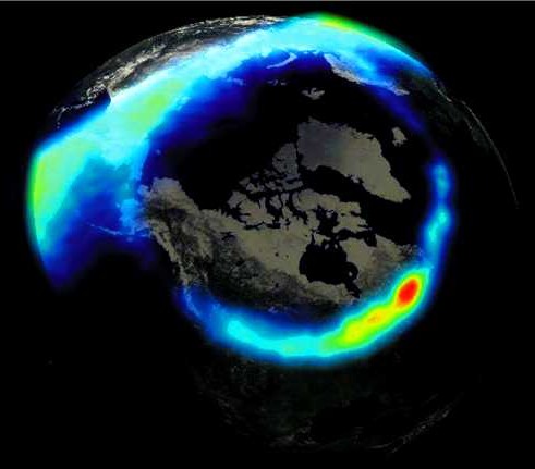
to add that the front cover has an absolutely fantastic photo of an
aurora taken from a satellite. There is a catch, however; the photo was made in Antarctica
and the book must be turned upside down to get the aurora positioned
over the polar cap. But like Confucius said, "A graphic is worth many kilobytes of
text."
Geomagnetic
storms and aurora
We
are now into disturbances of propagation, those nasty things that
can plague us, sometimes without our even knowing it. The last topic was magnetic storms and
aurora. Those represent disturbances of the F- and E-regions,
respectively.
The
effects of magnetic storms can be world-wide in the sense that
ionospheric electrons are removed from field lines, lowering the
MUFs on paths across great distances. The part of the ionosphere
which is disturbed the most is in the polar cap as that is the
region whose field lines are most at risk. And recovery from
magnetic storms is a slow process, requiring the electrons in the
F-region be re-supplied by sunlight, a slow, tedious process which
can take days after a severe storm.
The
effects of an aurora, by itself, are much more localized in the
sense that the increased ionization is confined to the field lines
that guided auroral electrons downward. Short of being in a full-blown magnetic storm, the effects
tend to be brief, measured in minutes or hours, and when the aurora
ends, it is a fairly rapid process. Essentially, the problem is to have the electrons in the
ionization recombine with the positive ions which were generated by
the influx of energetic auroral electrons.
To
listen: Auroral emissions
Audi
CD to buy: Auroral Chorus
I and II by Stephen P. McGreevy
But
now we come to solar proton events. Those will affect the D-region and originate on the sun, with
protons and other particles accelerated up to energies of millions,
sometimes even billions, of electron-Volts (MeV or BeV). So solar
proton energies, from acceleration on the sun, are
high in contrast to those of auroral electrons which are accelerated
locally, within the magnetosphere, up to tens of kiloelectron-Volts.
The protons are accelerated in connection with some solar
flares and then can leave the scene, passing through both the solar
and the interplanetary field.
The
interplanetary field generally points toward or away from the sun
and the outward progress of protons depends on the degree to which
they go along the field lines or perpendicular to them as they leave
the sun. But the
interplanetary field is not well-ordered like the geomagnetic field
close to the earth so protons will diffuse through the region and
their progress will depend on their momentum or the radius of
curvature of their path. The
more energetic protons will have radii of curvature which are large
compared to the scale-size of field variations so those protons will
follow more rectilinear paths. On the other hand, less energetic protons will have smaller
radii of curvature in the field and their progress will be more like
diffusion, scattered by the small-scale, organized portions of the
interplanetary field.
All
that is a way of saying that the high energy-protons will leave the
region close to the sun faster and make their effects felt more
promptly, albeit briefly. On
the other hand, the low-energy protons will diffuse slowly through
the field and their effects will be of longer duration. It should not
be forgotten, however, that the duration of the acceleration process is
of interest too. Generally, it is considered to be the same as the actual
flare process but those can be brief, in minutes, or longer,
measured in hours.
 |
|
 |
|
At
left, prelude to an intense auroral activity, this radioheliograph
reveals a strong eruption on the sun limb. It was
recorded on April 4, 2000 at 1342 UT at Nancay
Observatory. Emission came from the active region AR8948
and is directed straight to earth. At center the
unbelievable impact of the solar flux on the
magnetopause two days later by 16h UT. Click on the
image to run the animation. A right what happended in
the sky from April 7, 2000... The high atmosphere is
burning under the intense radiation emitted by electrons
discharging their energy. Documents Observatoire
de Paris-Meudon, S.M.Petrinec/Pixie
and Polar. |
|
Another
way of saying the same thing is if the flare region is off the to
the east of the solar disk, solar protons heading toward the earth
will have to stagger through the field lines which are more or less
perpendicular to their paths. That is a slower process and protons
can be held in the magnetic field region for times which are long
compared to the acceleration process that started them. As
an example, I had experience with one east limb event in August '79
where the solar protons finally reached the ionosphere 18 hours
after the flare! Staggering, diffusion? Yep!
On
the other hand, flare sites toward the west limb of the sun send
protons out into the field which generally trails behind the
rotating sun and we get "sprayed", as it were, by protons
going along the field lines. That is called the "garden hose"
effect. The Great Solar Flare Event of February 23, 1956 was a case in
point, a west limb flare where the travel time was measured in minutes.
Those were relativistic particles and had so much energy
(over 10 BeV) that they penetrated to ground level, even at the
magnetic equator! Been there, seen that!
But
what are their effects? Given the remarks in the last paragraph, one can expect
that the duration of the proton bombardment of the earth will depend on the location
of the flare site. That is one propagation clue that NOAA provides with every announcement
of a solar flare, the solar longitude involved. So that is one item of interest, east or west of central
meridian.
 |
 |
|
Map
of the D-Region Absorption Prediction. Compared to a
situation where there is not the least attenuation (at
right), it is rare that this map turns so red. It was
calculated on September 11, 2017, some days
after several sun flares of class X and M associated
to several emissions of CME by the Sun, among which
one was directed toward the Earth two days earlier.
When high energy solar particles reached the
geomagnetosphere, they affected a large part of the
ionosphere. That day, V/UHF bands
were closed at high latitudes with auroras in Alaska
and up to mid latitudes (>55° with Kp=8). This time the
effects of the CME created a radio blackout up to 15 MHz
where the attenuation reached till ~35 dB; a S7 signal
looked to a S1 signal ! You can get real-time update
on SWPC
website. |
|
But
as to the effects of the protons, those depend on their flux (or
number per cm2/sec) and proton energy. The low-flux, low-energy solar proton events were only
conjecture until the Space Age but are detected nowadays by
satellites and one can see the data in the Tiger Plots on a NOAA
website. But events with higher fluxes and greater energies can penetrate the
Earth's field and get reach into the ionosphere, the atmosphere and, on rare
occasions, they can reach ground level.
Our
interest, of course, is with ionospheric effects and being energetic
charged particles, the protons will leave a wake of ionization as
they plow through the atmosphere. The extent of the wake will depend
on the relative numbers of protons in the various energy ranges -
around 1 MeV, around 10 MeV, near 100 MeV and beyond. But
generally, being both energetic and massive particles as compared to
puny auroral electrons, protons penetrate deeper into the ionosphere
(if they get that far through the geomagnetic field) and the heavy
ionization near the end of their physical ranges can cause huge
ionospheric absorption of signals because of the greater
electron-neutral collision rate deep in the D-region.
For
solar protons to get down to the ionosphere, they must first enter
the geomagnetic field out at the magnetopause and then follow field
lines, according on their momentum. The present view of these matters is in sharp contrast with
the early days of ionospheric radio. Then, the dipole model of the earth's field was taken as the
standard and all discussions about the effects of solar protons were
based on work done by the Carl Stoermer, the Norwegian auroral
physicist. So the idea
was that protons were sorted out according to momentum (or energy)
by the field and there was a sharp cut-off energy which varied with
latitude.
|
|
|
Riometer
recordings of a PCA event reaching 6 dB over Macquarie island
(VK0, 54°S) on April 16, 2002. Document IPS. |
But with the IGY, things changed; the use of riometers,
looking at ionospheric absorption due to the protons, showed that
the cut-off idea was all wrong and the polar cap was wide open, full
of low-energy protons, all the way down to the auroral zones where
the cut-off energy was supposed to be 100 MeV. That was one of the first clues that the earth's field was
not that of a dipole; then measurements made by satellite-borne
magnetometers gave the final story, with the field configuration
I've sketched earlier.
The
coverage of the large polar cap area with solar protons is in sharp
contrast with the narrow latitudinal coverage of the auroral zones
by energetic electrons; beyond that, there is the difference in
levels of absorption, tens of dB on 30 MHz for solar protons as
compared to a few dB for the auroral electrons. So all in all, solar
proton events that reach the ionosphere, so-called polar cap
absorption (PCA) events, can be devastating when it comes to
propagation across the high latitudes.
But
there are few more aspects to PCAs to think about. For example, the
access for solar protons to the polar cap is one thing but it has
been found that solar protons can get into the magnetosphere via the
magnetotail. And the access to the two polar caps is not always
equal for solar protons, judging by satellite data. So there can be
different ionospheric reports from the two polar caps, depending on
sunlight on each and the access of the protons. All this makes
propagation interesting and confusing!
When
it comes to ham radio propagation, there is a propagation effect
that can mask the access to the polar caps. Here, I refer to the fact that there is a reduction in
ionospheric absorption in darkness, the number of dB in absorption
going down by a factor the order of 5 or so. This is due to the fact that the electrons created by solar
protons may attach themselves to oxygen molecules and form negative
ions. Negative ions are so massive that they do not participate in
the absorption process. So absorption in a darkened polar cap, at night or in winter,
is less and might be interpreted as a low proton flux without
satellite data to clarify the situation.
|
|
|
Riometer
recording of auroral absorption events during substorms that
occured on October 2, 1998. Documents DCS/IRP
Group. |
The
electrons bound in negative ions are released when sunlight is
restored to the D-region. That
is the case for proton events but not for auroral electron events
where the ionization is at much higher altitudes and electron
detachment results from collisions with atomic oxygen, abundant
above 100 km. So auroral absorption (AA) events do not show any day/night effect like
PCA events.
To
summarize now and put things in perspective: auroral absorption
events are limited in time and space, found during magnetic
disturbances, large or small. Polar cap absorption covers a wide
range of latitudes, the whole polar cap, and can last for days at
a time after some solar flares. And the ionospheric absorption is large, making PCAs a real
threat to ham radio communications. And if the polar cap expands in size in the late phase of a
magnetic storm, solar protons can then reach down to much lower
latitudes and have even greater effects of our HF propagation.
The
beauty of PCAs, if one would call it that, is that they are
relatively infrequent. The
real threat to ham radio communication is the effects of the solar
wind, so I would say that magnetic storming is the thing to watch
out for, by logging K-and A-indices to identify any possible
repetitions and then by checking each day by whatever means are
available. Magnetic
storming is THE threat to our peace and quiet; what the sun provides
in the way of higher critical frequencies by UV radiation can be
taken away in a jiffy by a blast of the solar wind triggering a
magnetic storm, minor or major.
So
monitor/log the magnetic indices; they hold the key to success in
high latitude DXing on the bands! But when the high latitudes are disrupted, try the other
directions, say across the equator. That is pretty safe, the field
lines there being shielded from the ravages of the solar wind.
And there's a lot of rare DX there to make things interesting.
 |
 |
|
Polar
Cap Absorption riometer profile recorded in Finland
(69°N) on April 21, 1998. The absorption increases when
the D-region is exposed to solar UV radiation, and this
day/night transition is a key feature for identifying
PCA in riometer data. PCA events are normally very
strong, often > 3 dB for sustained periods.
Auroral absorptions are much less intenses. Documents DCS/IRP
Group. |
|
This
is the end of the line and time to wrap up the discussion. It should
be in two parts, the theoretical side which we compare with the
experimental part. In regard to theory, the most general discussion would be one which
uses ray-tracing with the best available model for the ionosphere
and geomagnetic field. That is simple to say but as you know, words come
easy. But let's look at how it's done and what it means to
us. Then we can go to the experimental part.
Appleton's
magneto-ionic theory
Now
it may sound strange but the magneto-ionic theory that I mentioned
earlier is all cast in terms of frequencies. Obviously, the operating frequency is of utmost
importance. But then there are three other frequencies; how they compare
with the operating frequency (QRG) determines features of propagation.
The
first frequency is the plasma frequency; for a given position in the
ionosphere, it is another way of specifying the electron density.
Plasma frequencies in the lower ionosphere increase with
height, up to the F-region peak, and decrease with latitude toward
the poles. And, in a complicated way, they depend on the earth's magnetic field and
sunlight. But for signals to be contained, not penetrating into the topside of the
ionosphere, their effective vertical frequency (EVF) must be less
than the plasma frequency at the peak of the F-region.
The
second frequency is the collision frequency Fc between electrons and
the neutral constituents which surround them. As you know, collision frequencies Fc determine ionospheric
absorption and are greatest (<2 MHz region) in the lower
ionosphere. The comparison of interest is the operating frequency QRG and
Fc. If QRG >> Fc, then ionospheric absorption is not of great importance.
And a good example of that would be up on the 10 meter
band. But the plasma frequency is still of great importance as well
as sunlight on a path.
|
|
|
Electron
gyro-frequency between 630 to 1630 kHz. It is correlated with
the lines of the geomagentic field and MUF and affects the top
band propagation. |
The
third frequency is the electron gyro-frequency Fg, the number of
times per second an electron goes around the local field lines. For
the geomagnetic field, that ranges from 0.6 to about 1.6 MHz, in
going from low latitudes to polar regions as displayed at left.
And the comparison between QRG and Fg becomes very important
down on the 160 meter band as 1.8 MHz is comparable to values of Fg
along a path. The consequences of including the geomagnetic field in ionospheric
theory are very important and should not be overlooked in thinking
about propagation.
Before
getting to them, we should recognize that geomagnetic effects have
been neglected in almost all the discussion so far. True, it was
pointed out that the earth's field serves to keep ionospheric
electrons from running away, once released, but that was about it.
So for most amateurs, theory is quite simple: some
ionospheric absorption on the lower bands but otherwise, RF is
linearly polarized, depending on the transmitting antenna.
But all
that changed when Appleton embarked on formulating a more general
theory which included the geomagnetic field. The results are not to difficult to obtain but hard to
comprehend, given that the earlier theory is so deeply ingrained in
our thinking. But let's take a look at a few of them and see how things go.
First,
the strength and direction of the local magnetic field is important
and propagation depends on the direction of wave travel relative to
the magnetic field. That
is a new idea to most hams but is the case as in the more general
theory, RF waves are now elliptically polarized, depending on the
direction of propagation. That may be hard to picture so think of a
wave moving along with its E-field vector going around the direction
of propagation but with varying amplitude as its tip traces out an
ellipse.
Not
only are waves elliptically polarized but there are two types,
depending on the direction of rotation of the electric field -
ordinary and extra-ordinary waves. The two waves propagate with different speeds and, oddly
enough, are absorbed in the ionosphere (remember the collision
frequency?) at different rates.
Rather
than leaving things as they stand at this point, it should be noted
that the wave polarizations go over to simpler cases when
propagation is along or perpendicular to the field direction. To use
modern advertising parlance, there are also cases in the "not
exactly" category, quasi-longitudinal and quasi-transverse
propagation where the waves are close to, but "not
exactly", the strict limits mentioned above. That makes magneto-ionic
theory less stern and forbidding as the elliptically polarized waves are
close to circular or linear in those cases.
That
is a brief summary of what happens to RF when the QRG is comparable
to the electron gyro-frequency, say around 1.8 MHz. Added to that is
the idea of limiting polarizations where RF enters or leaves the
lower ionosphere. So there could be a mis-match between wave polarization
at launch and the limiting polarization at the bottom of the D-region.
In that case, the mis-match between the two polarizations
means the coupling of RF into the ionosphere is less than 100 %.
That is part of the "bad news" at the low end of
the amateur spectrum. Of course, there is also the question of the how the
polarization of the emerging wave matches that of the receiving
antenna. And the other
"bad news" is one mode, the extra-ordinary polarization,
is heavily absorbed over distance, meaning that more power could be
lost from that effect.
All
this emerged when Appleton worked through the more general theory of
how ionospheric electrons respond to RF in the presence of the
geomagnetic field. Once
that is done, the next step is to incorporate the results into the
"equations of motion" for waves and do ray-tracing with
the best field model available. The consequences are interesting, as you can imagine, with
the important result that ducting is possible just with the typical
electron density gradients present in the ionosphere.
All
this is probably more than you wanted to read about but you should
know that the simple ideas that are abroad are not the final story.
But one idea from magneto-ionic theory that applies at
frequencies way beyond the electron gyro-frequency is the rotation
of the plane of wave polarization.
|
|
|
The
Faraday rotation can be measured in placing a linear
polarizer on each end of a solenoid containing a
transparent material and cross them at 90°. This rotation
angle can be measured as a function of magnetic field, length
of sample and wavelength of light. |
Ordinarily, changes in HF polarization are attributed to
ionospheric tilts, not an effect from the magnetic field. But it is real, seen with satellites on
VHF.
The
idea comes from sending linearly-polarized signals along the field
direction. If you think
about it, a linearly-polarized wave is the same as the sum of two
circularly polarized-waves of equal amplitude but rotating in
opposite directions. The
rest is straight-forward as the two circular polarized waves travel
with different speeds, meaning that one gets ahead of the other, and
the polarization of the resultant linearly-polarized wave is rotated
as it travels along. That
is Faraday Rotation and is an important part of work on VHF where
two circular polarizations can be present with essentially equal
amplitudes.
But
a problem with Faraday Rotation comes up on the lower bands as the
extra-ordinary wave is heavily absorbed and over any great distance,
the ordinary wave is the only one that survives. So it is not so much a question of Faraday Rotation on 1.8
MHz but one of the remaining ordinary polarization and how it
compares with the limiting polarizations at the bottom of the
ionosphere and antenna polarizations.
As
for the experimental side, that really deals with what we know about
our surroundings. Starting
from the ground and going up - the geomagnetic field, the neutral
atmosphere, how solar radiation affects the atmosphere and creates
the ionosphere, the solar wind and its effects on (or in) the
earth's field, the solar magnetic field and solar activity. There's
a lot to know and more to the point, it's important
to appreciate that we're dealing with a coupled system. So any
effect that is dealt with in isolation may not be well
understood.
The
present situation as far as propagation is concerned depends on the
use of computers and that brings up the question about the programs
that are available. For
the geomagnetic field, there is the International Geomagnetic
Reference Field (IGRF) while the models of the ionosphere are found
in the Internation Reference Ionosphere (IRI-2001
at U.Leicester and at NSSDC). Those two serve as research sources but also find their way
into software such as PropLab
Pro or DXAtlas.
Then
there are also the various propagation programs that are available
at present. Viewed by
themselves, they are efforts done in isolation with quiet-day
representations of the ionosphere. So additional consideration must be given to the details of
the critical frequencies all along a path and also the geomagnetic
circumstances and any unusual ionization, say from solar protons.
That's where mapping programs and the SWPC websites on the Internet
prove their value. Without
using that information, it is hardly possible to make a realistic
prediction of anything.
As
an example, the week of Nov. 8-14 was characterized as one of
considerable magnetic activity and solar activity. Thus, the following A-indices were reported from the Boulder
magnetometer: Sun: 68, Mon: 78, Tues: 6, Wed: 4, Thurs: 4, Fri: 60,
Sat: 38
Without
that knowledge, the results for propagation conditions from a
computer program, using only input with regard to sunspot counts,
would make you think you live on a different planet as they would
have little bearing on actual conditions.
Top
50 solar flares, Spaceweather
 |
 |
|
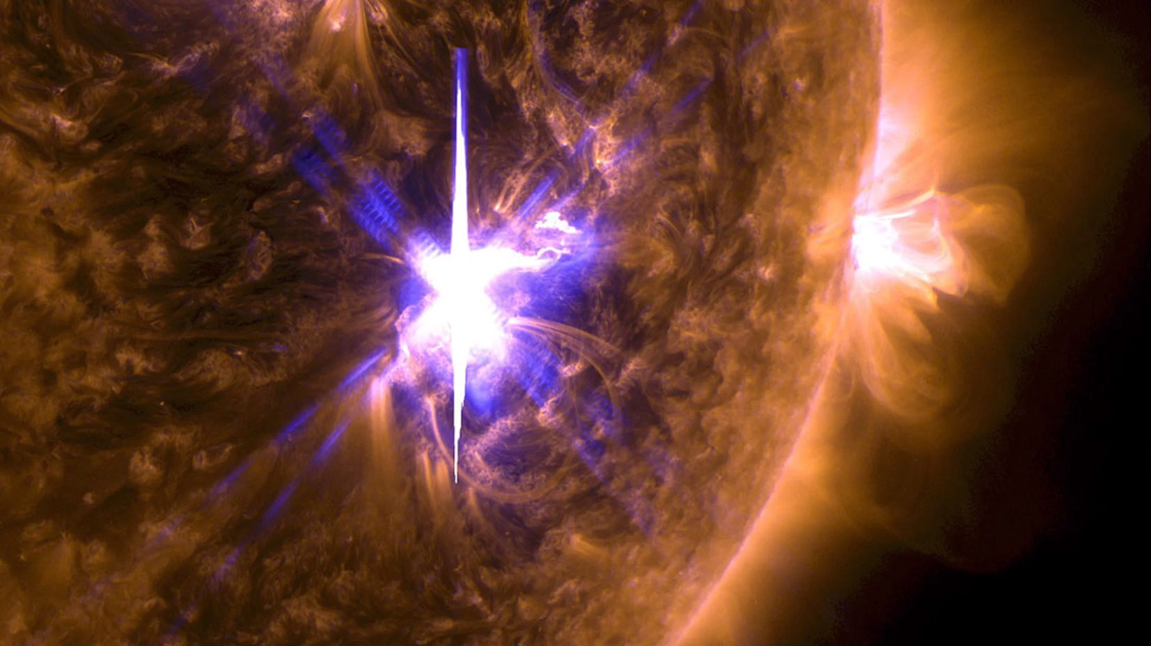
At
left, a picture recorded by SDO
in EUV at 131 and 171 Å of a chromospheric eruption of class
X9.3 occuring on the Sun on September 6, 2017 between 11:53 and 12:23 UT in the active region
AR
2673. This was the strongest since September 7, 2005 (class X18). It
was associated with the emission of several CME and
several other sun flares in the next days. At right, a
coronal mass ejection (CME) disturbs solar wind
currents and creates magnetic disturbances that hit
sometimes the earth in a catastrophic way. The
Wide Field and Spectrometric coronograph LASCO
onboard the SOHO
satellite has observed many CMEs. The spectacular
event of September 12, 2000 displays above created a
halo event giving the feeling that the whole sun was
surrounded by the CME. Such halos are generated by
sunflares (eruptions) directed toward Earth.
Click on
the image to run the animation (.GIF of 595 KB).
|
|
But
that is not the whole story as the CME that was responsible for the magnetic
activity also produced a solar proton event on November 14. Then, 10 MeV protons,
which are capable of reaching the ionosphere, appeared at satellite altitudes
around 0600 GMT. The proton flux peaked at 300 p.f.u. (proton flux units or
protons/sq-cm/sec/ster) around 1245 GMT and continued coming out of
the interplanetary field for more than a day. Also, there was a weak flux
(6 p.f.u.) of 100 MeV protons, capable of reaching balloon altitudes
(about 30 km), was present. In addition, there was a strong increase in 1-8 A X-ray
background on the 13th.
As
I said, these are coupled systems and we have to look at more than
one limited aspect if propagation is really our interest. Of course,
as we go toward solar maximum, this will be the case more and more often. But
on the cheery side, the week of Nov. 8-14 has to be an exception.
For example, in the year that I spent in my long-path study
around the maximum in Cycle 22 , something like 80 % of the days were
free of any significant disturbance and even with minor or major
disturbances on the rest of the days, I was able to make a long-path
contact on over 90 % of the days.
That
suggests a cautious but optimistic approach is called for, watching
all the disturbance indicators on a regular basis, "going for
it" when propagation looks good and even "looking
around" when conditions may not be the most promising.
I like to say "DXing is an intellectual pursuit" so
it's worth a bit of study; that makes the rewards all the more
enjoyable.
Conclusion
I think I've said all I wanted to so let me close with words of a
great man that I'm sure you'll recognize: "That's all
folks!"
73,
Bob Brown, NM7M (sk)
For
more information
On
this site
PDF
version of this document (for printing purpose, without images)
Real-time
status of solar, geomagnetic and auroral activities
What
can we expect from a HF propagation model ?
Review
of HF propagation prediction programs
On
the web
SWPC
An
Introduction to HF propagation and the Ionosphere, ZL1BPU
Radio
wave propagation (chapter 2), TPUB
HF
Radio Propagation Primer, by AE4RV (Flash presentation)
ON5AU's
Propagation pages, Marcel De Canck
Introduction
to HF Radio propagation, PDF file from IPS, released
in HTML format at G3YRC Radio Club
or N1QS
Propagation
Studies, RSGB
ARRL'
Shop
RSGB'
Shop
The
DX Magazine
Books
Propagation and Radio Science,
Eric Nichols (KL7AJ), ARRL, 2015
The High-Latitude Ionosphere and its Effects on Radio Propagation,
R.D.Hunsucker/J.K.Hargreaves, Cambridge University Press, 2007
Physics of the
Upper Polar Atmosphere, by A. Brekke, John Wiley & Sons Inc,
1997
The
Little Pistol's Guide to HF Propagation, by Robert R. Brown
(NM7M), Worldradio Books, 1996
The
New Shortwave Propagation Handbook, by Jacobs, Cohen and Rose,
CQ Communications, Inc., 1995
Radio Amateurs Guide to
the Ionosphere, by Leo F. McNamara, Krieger Publ.Corp.,1994
Ionospheric
Radio (IEE Electromagnetic Waves Series, Vol. 31) by K.Davies, Inspec/Iee, 1990
Radio
Wave Propagation (HF Bands): Radio Amateur's Guide, by F.Judd,
Butterworth-Heinemann; 1987.
Back
to Menu
|


