|
Software review
DX
ToolBox propagation analysis and prediction program (III)
Propagation
Map
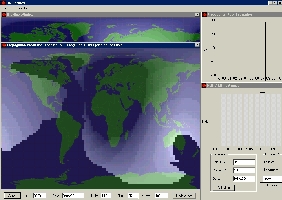
The
“Propagation map” window displays an estimation of
propagation conditions at earth scale rather than between
two stations. A gray scale is incrusted on the world map
centered on your home location, which brigthness and extent
depend on all involved parameters.
The
required information are the solar flux, the working
frequency expressed in MHz, the transmitter power level
expressed in Watts, the date and time in UTC. Some of these
data can be extracted from the “Current Conditions”
window in pressing “Now” or entered them manually to
simulate another time and/or another solar flux.
Once
this information entered, press the “Update Map” button
to get an estimation of the propagation. This forecast
displays also in the upper bar the estimated signal strength
in dB and the number of hops between your “home”
location and any location pointed on the map.
The
system makes the assumptions that the receive bandwidth is
about 2.5 kHz, and the minimum sensitivity of the receiver
is -123 dBm (~2 μV), typical for most modern receivers.
 |
 |
|
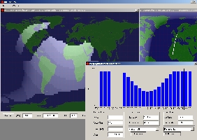
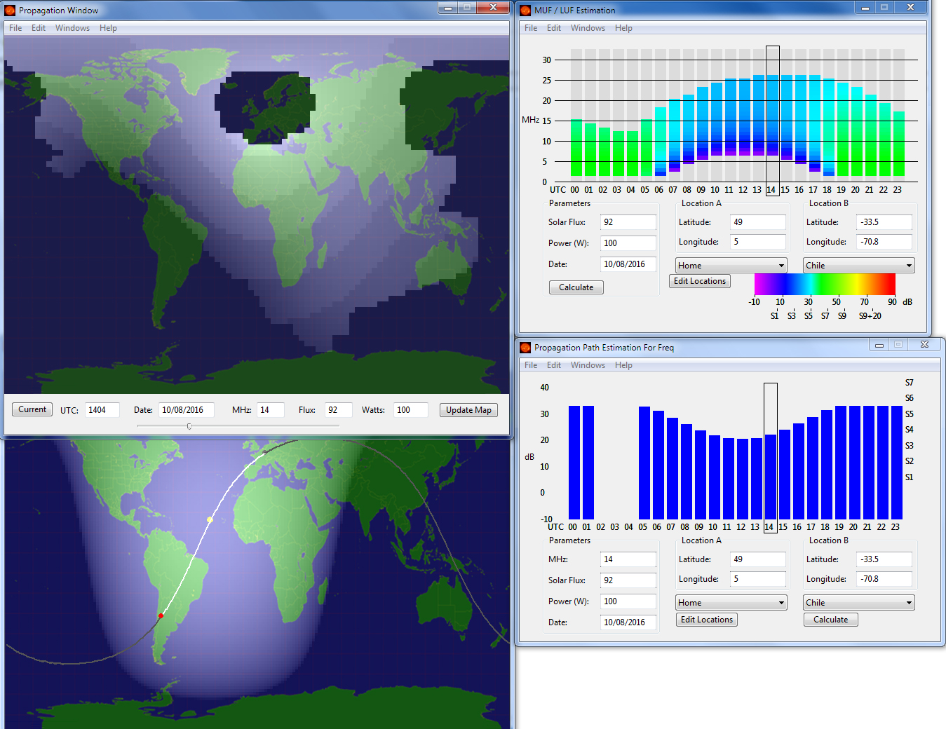
The
“Propagation Map” and charts calculated with DX Toobox. At left, for a
circuit between LX and CE on August 2016 using a
vertical antenna in SSB with 100 W. At right, another
prediction calculated for the 20-meter band for a
circuit between ON and VU for August 2004. |
|
This
map uses an increment of 1 hour only; the forecast of 1030 UTC for
example is thus the same as the one of 1000 UTC or 1059 UTC;
it a pity because you have no possibility to
"intercept" a sudden opening in real-time like
that occurs quite regularly on the low bands. The same step
is used to display the propagation chart. Of course no one
program is today able to take into account real-time conditions. But
it should be interesting that a forecast is be able to predict
opening in a time-lapse shorter than one hour.
This map is also an educational mean to understand what is
the skip distance (or silent zone displayed in dark gray) around your emitter according the
frequency used or to know how many hops there are between your
station and a remote one.
This
window cannot be adjusted, only moved or closed, and fills the 2/3
of an SVGA screen. It is thus superimposed to the Grayline map or
any other chart and you cannot always click on some area hidden
behind other windows. This is annoying when you want to display
several windows (even with two it is a problem) or run
simultaneously another application as it will fill at least half of
you screen as well. A variable-size window should be welcome and
very appreciated.
The
accuracy of the prediction is however more than disappointing as the
system uses very few inputs and
simple ionospheric algorithms. The propagation map works better on
the highest frequencies with a high solar activity. It also displays
from time to time some minors bugs like a thick black line across
the middle of the screen or displays a "No reception
possible" message in an area close to a silent zone (dark gray)
but where the propagation is still open (signal stronger that -12 dB
below which it is considered as lost by the program). These small
"bugs" that do not prevent you to use the program should
be corrected in a next release.
Propagation
Chart
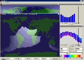
The
“Propagation Chart” window displayed below pops up in fact each
time that you request a Propagation Path Estimation in clicking a
location on the Gray line or the Propagation map.
|

|
|
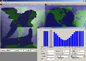
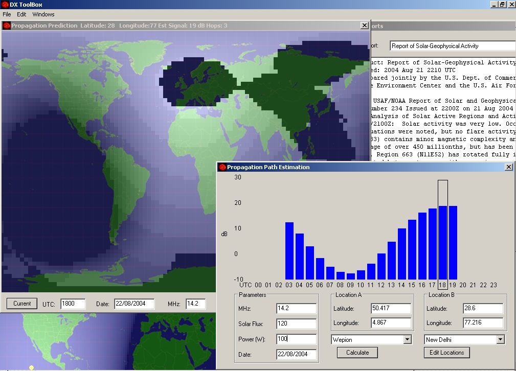
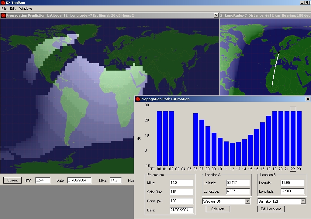
The Propagation Chart displays the signal
strength in dB between the location A (usually your home)
and any location B when you click somewhere on the
Grayline or the Propagation map (in this case in the
area YI-HZ). The wired black rectangle at right highlights
the current time (UTC)to the user (location A). |
Preset
to use the current conditions data, the “Location A” is the
location that you set in the Preferences (your home usually), while
the “Location B” in any station pointed on the map or
coordinates entered manually.
This
is in this window that you can simulate other times and solar flux
entering their value manually.
Following
whas has been told about the accuracy of the Propagation map, using
the same algorithms, this chart displays obviously the same
limitations as it displays the same forecast, but no more at the
global earth scale (area coverage) but between two stations (point
to point); the propagation to some DX looks for example open with
a strong signal over 15 dB and a MUF well above your working
frequency but in the field, at the radio, the ears tensed or the mike
warming, you cannot either work any station nor hear the beacon
located in that country; another factor not considered affected the propagation.
Hopefully,
at other times the forecast matches the real conditions
but I cannot say exactly yet in which conditions values reverse the
prediction from reliable to not reliable, all the less that the
reliability is a term unknown from DXTB.
Of course the frequency
used and the solar flux level are the main concerned factors but it
is hard to say what is the triggering level : probably when the sun
enters in a quiet cycle (SSN < 100), at low frequencies (14 MHz
and below) where forecast becomes less accurate, and also at
distance longer than 6000 km, triggers to confirm in the
field or if we know what algorithms are used.
The
bar-graph shows also sometimes one or more missing bars : this is
not a bug but a drop in the propagation (see below). This chart
using a 1-hour increment, the decrease and increase of the signal
strength fall between two steps and thus they cannot be displayed to
smooth the "curve".
Neither
the propagation map or the chart takes into account the ground
properties (conductivity and dielectric constant) or the change in
propagation along the gray line. Yet, these factors affect the
radiation pattern and the maximum range of your antenna. A simple
example : if you can easily reach VK for K as most of the circuit is
over the sea, it is much harder to reach JA from ON through Russia.
Idem with the gray line that helps much for DXing.
In
my last mail to the publisher (August 2004) I suggested him to use a
smaller incremental step, trying to use the ground properties in
forecasts, to add more series in this chart, like for example the signal
strength as seen from the receiver at night, the signal-to-noise ratio and reliability, the
best usable frequency or other custom series. At last the format
could be customized too, allowing the user to select the colors and
the chart type (bar, line, area, etc). An alternative is using a color
mapping as he does for the MUF/LUF estimation (see below). Of course
some users will prefer bars while other will prefer the rainbow, but
the choice should exist.
Locations
Window
|

|
|
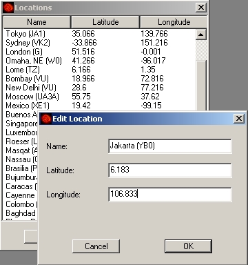
The
"Locations" window. |
This
window is only available through the Propagation or MUF/LUF
Edtimation Chart. Logically it should be available from the main menu
("Windows") as well, what I suggested to the publisher.
By
default DXTB provides no location contrary to other applications
that list several thousands cities worldwide.
If
you click on the “Edit Locations” button, a new window
pops-up in which you can add, edit or delete locations. The program
is limited to a maximum of 100 locations without accentuation. Don’t
forget the minus (-) sign when encoding southern latitude
and western longitude. Type also the coordinates as decimal
integer with the decimal point (.) even if the
"Preferences" display a coma (,). If you enter a
coma the program reacts stupidly, display a black vertical
line in the middle of maps and shuts down (bug). If you
type well a dot, you’ll need to close and re-open this window
for the changes to take effect.
The
three columns can be sorted but it always didn't work in the
release 2.2.0 under Windows XP or ME. New cities added were not
saved each time neither, and I had to retype them several times
for the change to take effect.
To
add conviviality, I have suggested to the publisher to correct these
bugs, to insert a "refresh button", to permit the user to
encode angular values on request as he does for the QTH locator
(grid), and to provide in a next release names and coordinates of
main international cities.
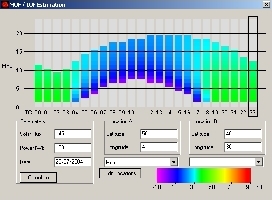
MUF
/ LUF Estimation
The
“MUF / LUF Estimation” window allows you to estimate the signal strength for a specified path for a
range of frequencies over which propagation is expected or
impossible. Recall that the MUF is a statistical value representing
the median value of the predicted propagation estimation.
But this prediction alone does not tell all the story.
|
|
|
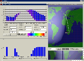
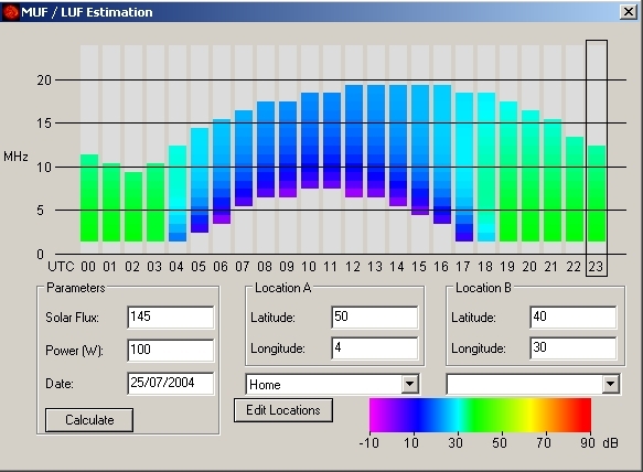
The
“MUF / LUF Estimation” window for a path
from ON to TA with 100 W PEP. The propagation looks open with
signals at night 40 dB higher than at daytime where low ionopheric
layers absorb signals. Such signals are common at short distances. |
MUF
and LUF strongly depend on the solar flux, the transmitter power,
the time of the day and of the year as well of the location of the
transmitter.
You cannot
simply trust in this forecast to plan your QSO
because any geomagnetic storm will also affect the
propagation of your signal, and thus the MUF, as well
as the S/N ratio associated to the
bandwidth of your operating mode while the D-layer status
will affect the LUF. It is thus a chart rather complex to
interpret without more information, all the more that it
displays simultaneously three variables as a time function :
LUF, MUF and the associated signal strength estimation in
the scale at left expressed in dB or its equivalent in the
rainbow meter.
If
you understand well what represent LUF and MUF, this
chart is then very useful and it is also user-friendly. The
color mapping based on the rainbow colors ranges from
purple for the weakest signal to red for strongest signal, the green being in
the average. This color mapping is really efficient and speaks by
itself, as good as the Propagation Chart bar-graph expressed
in dB.
More
interesting, you can bring this window up by holding down the “Shift”
key while clicking on a location on either the Grayline or the
Propagation Map window.
I
think that the capabilities of this color mapping associated to the
signal strength could be pushed much further to provide more dynamic
forecasts displaying for example the SNR, S/I ratio, reliability,
etc, if these parameters could be taken into account by more
accurate algorithms.
Grid
and Grid Map
At
last the Grid calculator lets you determine the grid square (QTH
locator) from the longitude and latitude. You enter them as decimal
integer values or using the degrees, minutes, and seconds. The given
value is correct.
The
“Grid Map” windows shows a map of the world showing grid square
and time zones at large scale. You cannot browse it except to
enlarge it in full screen and moving inside with the lifts. If you
move very slowly the mouse over your QTH locator you can find it but
its resolution is perfectible as the way to move on the map.
Accuracy
of forecasts
In
buying DXTB, the amateur expects to get accurate forecasts.
But he also knows that buying this program at the
price of a good book about propagation these predictions
could be as accurate as astrologers' ones. On the other
side, a more complete model like VOACAP is free. So what to
think about the accuracy of DXTB against the one of its
competitors ? What reliability or degree of confidence can
we grand to such a program ?
Except
the common inputs, SSN, geomagnetic indices, the frequency, the
date, time of the day, and the power, you cannot ask the program to
take into account an additional variable. DXTB doesn't take into account either
parameters of a complete circuit (ground, transmitter, antenna, tolerance, S/N ratio,
reliability, etc) nor the operating mode or the hop structures. As
all these inputs are bypassed, it only works with the ouput power, a
predefined receiver sensitivity and raw assumptions about the propagation
mode or the signal strength injected in simple ionospheric models like
Fricker's MUF and F2-peak models. But without considering many data, the
results can only be biased, and therefore DXTB cannot thus gives you an accurate
prediction for a specific path but only "the big picture" with some percentage of confidence.
 |
 |
|
|
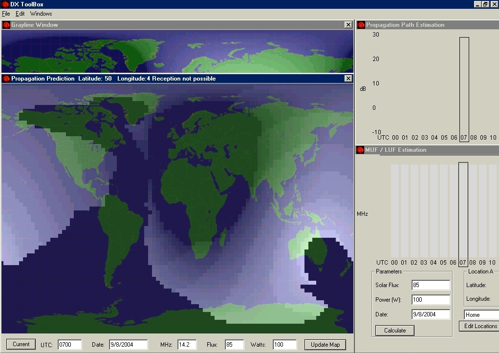
DXTB
predictions compared to the ones of the "golden
standard", VOACAP. Above propagation conditions to Europe as
seen from Australia (Canberra) on 20 meters for
September 2004 at 0700 UTC (SSN = 27, SFI = 85). DXTB
predicts no reception possible in Europe and Canberra
is in the
silent zone. It is unable to predict the MUF/LUF and
forecasts a S/N below its threshold of -12 dB (both
windows displayed at right are gray without the least
bar). At right, VOACAP set for the same date and SSN,
for a Yagi transmitter side with 8 dBi gain and 100 W output,
a S/N reliability of 73 dB (SNR) and a required
reliability (SNRxx) of 90%, thus good signals and
conservative values. It
predicts some opportunities between 06-09 UTC around
14 MHz with a signal strength at receive between -145
and -150 dBW or S2 and a S/N of 25 dB, thus weak. In
the field VK/ZL stations arrived on my 2l
dipole between S1 and S4 with a weak to strong audio,
values that matched VOACAP predictions but not at all
the ones of DXTB. Below, the same imprecisions occur
when one tries to predict propagation conditions on
evening. |
 |
 |
|
Above
a forecast
calculated for Belgium on
August 5, 2004 at 2200 UTC on 20 meters and 100 W
output. The audio reports match partly the prediction from DXTB : signals from FY
stations matched. LA or UA stations, so-called
unreadable, were as strong as FY. K and XE were still weak
but could be worked. The MUF over New York is
predicted close to 9 MHz where VOACAP predicts it
higher, close to 11.5 MHz at that time (not shown). At
right calculated for the same time VOACAP predicts for
UA (Moscow) a signal
strength of -140 dBW or S3 and a S/N ratio of 27 dB;
UA will be weak but could be worked contrarily to what
states DXTB. Differences between DXTB and VOACAP come
from the fact that the first does not consider either the
path, ground properties,
antenna gain or the reliability, but uses only median
values, good for an overview but far to be enough to
give an accurate forecast for a point-to-point
circuit. |
|
DXTB
is for example unable to predict a drop in the propagation (strong
QSB for tens of minutes) or a gradual increase of the signal due to
a change in the LUF at daytime. It predicts well a global change in
the propagation at earth scale (closing down or opening with an
increment of 1 hour only) but it doesn't see these small variations
that a program like VOACAP for example can predict
As
DXTB does not let you select the parameter to display (there are none
except
the propagation estimation per band, MUF/LUF
associated to a power strength meter, and a point-to-point
signal strength meter), you have to
trust in the dB scale, the color mapping or the signal strength
meter displayed in charts. Impossible to know the parameter
reliability or whether the value displayed is a
median (like the MUF I hope), a low or a
high probability (e.g. a high or a lower decile, etc).
This
application provides no access to curves like FOT, BUF and HPF (we
can estimate them of course), there are no cross-sections of the ionosphere
to get an accurate view of the height of the ionospheric layer(s)
used in the circuit, no iso-contour or global maps showing critical
frequencies (MUF, LUF, F2, etc), not even a S/N ratio or a power
signal decile chart.
In fact you
have no mean to know whether the forecast is right or false or to
discover slight variations in propagation. In
other words your unique way to know the accuracy of the prediction
is to switch on your radio to check if the signal of the DX station that you hear
or are going to work fits well in the estimation calculated by the
program.
This
inaccuracy appears quite rapidly when you request a prediction. In
the Propagation map, DXTB refuses for example to consider the
possibility to work at 100 W PEP a station located at short distance, say 1000 or
2000 km away (1600-3200 miles), at night on the 20 or 17-m band in
summertime. Even without using a computer but only understanding the
propagation fundamentals, there are of course several objective reasons to deny
this QSO (season, D and E layers vanished, skip distance, low solar flux, in other words a
band almost dead or experiencing strong QRN and QSB).
But in the
field you will observe quite often that the band is not as closed as
estimated and even on clusters amateurs spotted some contacts. The
same inaccuracy appears with DX stations (located over 6000 km away)
that are estimated too weak to be heard ("Reception not
possible") and who arrive quite strong and that can be work
using a beam.
But
usually silent zones represent well what they are : an area in which
there is no propagation at the specified time, frequency and power.
Hereunder is an example showing the propagation chart from ON to TZ
(Mali). The "missing signals" between 0300-0500 UTC are real,
correlated with the silent zone associated to the darkness on this
part of the earth at that time.
 |
 |
|
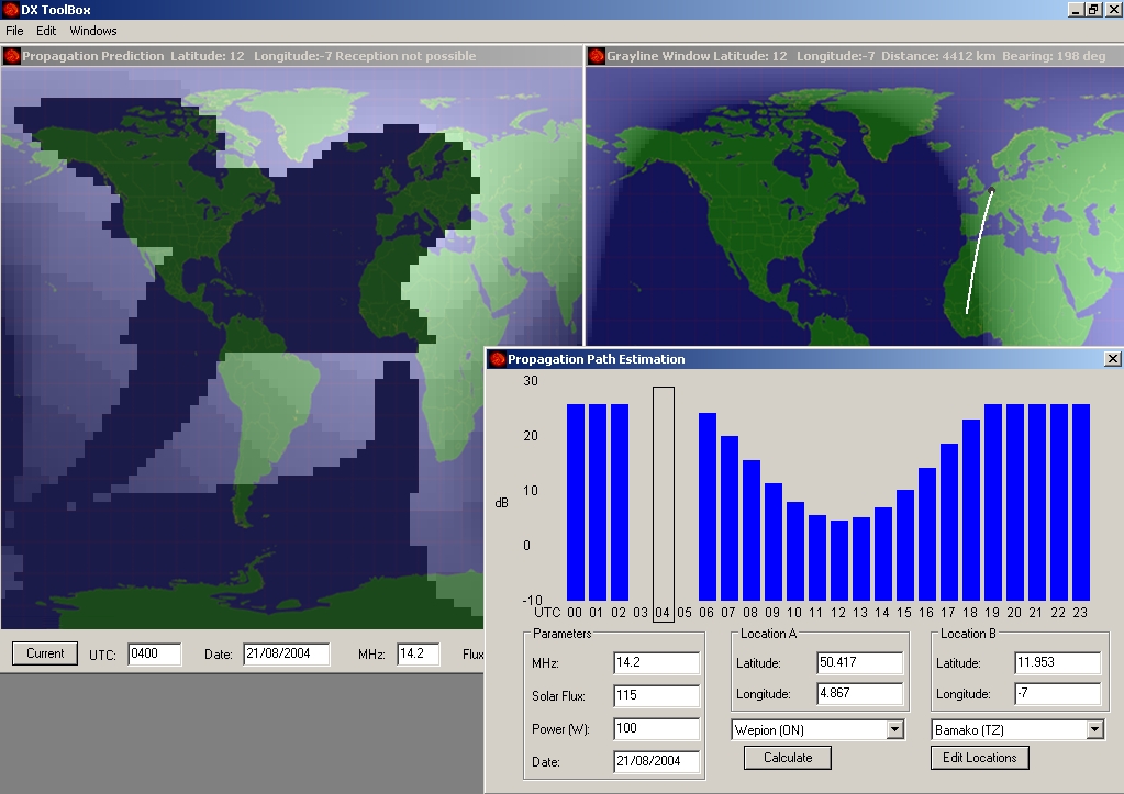
Propagation
chart calculated for August 21, 2004 at 2200 UTC
(left) and 0400 UTC (right). I ran the simulation
earlier to understand the reason of the void (no
signal or lower than -12 dB) in the propagation chart
between 0300-0500 UTC. This is not a bug but a real
effect related to the silent zone associated to the
darkness over TZ in these early morning hours. |
|
Well,
and at the end, if a forecast states that the band is closed, is it
really closed or not ? In fact this
problem concerns as much the operator's working conditions (his/her
antenna system and the mode used) as the propagation : even if the
propagation is so-called closed, a beam could still reach a DX
station where the omnidirectional vertical gave up for a long time.
If you add some power, that will be
still easier, and still more if you work in CW. However, even if
DXTB takes into account the power, nobody tells it either that you
use a high gain beam placed 12m high or an isotropic antenna at low
height for example, or that you work in CW. These factors affect
thus the prediction of a serious bias.
This
dependency on the working conditions is obvious checking beacons that transmit without
interruption in CW. In the Propagation map, DXTB displays more than once "Not reception possible" at daytime
with a signal strength below -12 dB (thus "below" the
first S-unit) although the beacon is very
strong at 100 W (ZL6B reached S-7 and ZS6DN was S-5 during hours);
at other occasions it forecasts a strong signal (+18 dB) at daytime
although the beacon located a short distance was unreadable (e.g. 4X6TU or RR90). In most of
these cases, but not always, at the specified time the MUF, LUF and
signal strength are simply not
displayed because the program considers the signal too weak (what usually means that
the darkness is not far but the contrary is also true, or that the MUF is lower than the working
frequency or, at daytime, that the D-layer is still too active, but
many other interpretations are possible).
 |
 |
MUF/LUF
estimation, propagation and signal
strength forecasted for ZS6DN beacon at 1127 UTC (left): no signal to
expect in ON. At the earth scale, in the propagation
chart displayed in the below right corner it was obviously confirmed : there was no propagation (dark
gray) to South Africa. However, at the radio the 100 W
beacon arrived S-5 on a simple
dipole 40m long ! By 1800 UTC (right) the forecast
predicted a much stronger signal exceeding 10 dB and
the propagation chart below right confirmed a strong
signal (+12 dB) up to South Africa. That
matched: this time it arrived S-3 with a strong audio. |
|
Most
of the time, as you have no other chart at your disposal to cross-check these
values (especially the median S/N, SNR, receive antenna properties,
signal power lower decile, etc) you stand in ignorance of the real reason that led to these lost of
propagation or sudden openings to such or seach country. This is not really the objective of
a propagation program that should highlight the true reason of these
poor conditions (showing a signal strength in the purple, a very low
power at receive, low reliability, or conversely a strong signal, high SNR, low
losses, etc).
The
problem is emphasized by the fact that you must also interpret
graphs and figures, although a map or a chart is by definition
self-explanatory. But even if a green color means "good signal" or if a signal strenght of
10 dB looks strong, 10 times stronger than a 0 dB signal, it
does not mean much as long as you don't hear it in the reality. Add
also the fact that this interpretation acquires also with experience
in working on the air, still the best way to try correlating what
you hear with what state, with more or less accuracy, maps and
figures. In all cases to explain a
changing propagation, display always both Propagation and Grayline
maps together, because if the information is not self-explanatory on
the first map or in its chart, the second one will give you some
clues. Another trick is to run the Propagation map some hours
earlier or later to see how it changes, knowing however that such a
program is not really suited to work with short-terms but rather
with longer lapses, of one or more days.
|
|
|
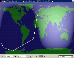
Trying
to set a prediction for a long path to
VK/ZL, at the limits of the map (52°S, 176°W) DXTB traces a
surprising path. |
Knowing
all this, we can say that where other propagation programs lack of
parametric maps to cross-check predictions, DXTB lacks of additional charts to
validate forecasts. But we have to put all these problems into context
because, as we told, other more sophisticated programs display also some degrees
of imprecision. Reasons are known and multiples : all these programs
use algorithms more or less accurate, with or without interpolation,
or use functions extracted from the same ionospheric model and set their probability or their
degree of reliability to median values.
At
last, we explained earlier that DXTB shows also some errors at
the limits of maps. Stressing the program, I tried to display the long path to New-Zealand
and Australia, and the concerned propagation chart.
Impossible, the function is not supported. Annoying when you
want to work VK/ZL using the long path from Europe (say
between 0400-0800 UTC) to benefit of the darkness and a stronger
signal...
If you select
an island close to ZL and the left frame, at
some coordinate points located near 52°S and 176°W, very close to the frame, the
path is erratic, it begins to shows steps instead of a smooth
curve. The function has been improved and does no more shows straight lines and steep angles instead of
a curve like do other applications (remember that we work with
geodesics). But the reason of this error is obvious : many
programs doesn't take very well into account conditions at the limits,
especially the high angular values at high latitudes due
to the cartesian projection. I suggested to the publisher to
still improve the display accuracy and to
add a long path calculation.
My
final impression
A
lot of features are available in “DX ToolBox” at a few
keystrokes. Not only it is cheap and good-looking but it provides a
very intuitive graphic interface with maps, charts, images and
reports that will satisfy all casual amateurs and even amateur
astronomers who are looking for near-real-time solar and geomagnetic
bulletins.
If
you want to understand the behaviour of the ionosphere and figures
listed in bulletins displayed on-screen, its “literature” is
made for you, I mean all its warning messages and other status
available in its "Reports" window. In addition tens of
images, including your own links, will illustrate its most verbose
text. And all this is accessible simply in clicking in one submenu.
Time consumed : a few seconds once all images and reports and
downloaded. Even forecasts display quickly. That cannot be simpler
and faster !
This
simplicity has unfortunately a drawback. The engine hidden behind
this program, algorithms or functions, are not as numerous, flexible
and powerful as the ones included in a coverage analysis program
like the VOACAP model for example. Its
accuracy is thus limited. But as we told, as well as in other pages
dealing with the ionospheric
modeling, many other programs in this category show restrictions
too, and either VOACAP or DXTB doesn't go against the rule.
So,
without to be either powerful nor a complete tool, DXTB covers most requirements
of a casual amateur and will probably please to the advanced DX addict
amateur looking for a simple propagation program. However; much cheaper than more
sophisticated programs using the VOACAP engine, do not expect the same
accuracy and the same functionalities as its competitors.
But
positive side, if you don’t understand anything at all in the
propagation, I make the bet that thanks to its online reports and
dynamic windows this program will help you to understand better this
complex subject, and that you will do a big …hop ahead, Hi !
Download,
purchase and support
“DX
ToolBox” is now at version 4.6.3. It is available for all Windows and Mac platforms (incl. OS/X, iPhone, and iPad). It requires an active Internet connection for get online updates.
“DX
ToolBox” is free to try out and can
be downloaded as
an installer or a compressed Zip file from the
publisher website, a file that "explodes" in about 13.1 MB of data distributed in five
files. Some of its competitors are over three times bigger
without offering more accuracy.
In
this “free to try” version it displays at regular interval a
warning message. If you decide to continue using it, you can buy a
copy for just $24.99, which gives you a registration code to remove
the reminder messages (code to enter in "Edit" menu, "Enter Registration
Code").
“DX
ToolBox” runs on a single computer. If you wish to run it on
multiple computers simultaneously, you must obtain a license for
each system, or the appropriate site license. Please contact Black
Cat Systems for pricing and details about site licensing.
Last
but not least, when you purchase you'll be entitled to use all new
releases and updates to “DX ToolBox” released over the next
year, free of charge.
Close
this review saying that
the response of Chris Smolinski to users enquiries is fast at first
contact and comes back with tips and a fix less than 24 hours later.
This is very appreciated when you are face to problems.
Congratulations!
I hope that you will appreciate
this product.
Last
note from the publisher, Chris Smolinski
July
26, 2004 : "Thanks for the suggestions, I'll consider
them. I also am in the process of writing a brief tutorial on
propagation, what the various indices mean, etc". This tutorial
is already partly available on the publisher website (see below).
For
more information
If you are seriously interested in
propagation, I warmly suggest
you to read some books and studies
that you can find in the ARRL or RSGB bookshop. Completed with
simulations, you will become
without any doubt a guru in this matter, Hi !
DX
ToolBox propagation software, Black Cat Systems
HF
Shortwave Radio Propagation Information, Black Cat Systems
HF Propagation tutorial, NM7M (on this web)
Propagation
Studies, RSGB
ARRL
Bookshop
RSGB
shop
Back
to Menu
|


