| Spectra data reduction |
Spectra data reduction
![]()
| The spectrum pre-processing consists into several steps to transform a set of raw acquired images into a calibrated profile.
Two main steps are followed: - pre-processing to convert raw images into one combined image with bias, dark and sky subtracted spectrum, using IRIS - no flat-field have been made during the observation sequences - spectral calibration: wavelength and some flux normalization with a reference star, using Visual Spec Another description of the spectral data reduction is available in a power-point presentation presented at the 8th astrophysical school of Oleron, CNRS: click here. |
| Pre-processing |
| Usually a sequence of 10 to 20 images are acquired. In addition 10 offset images and 10 dark images are acquired during the night. |

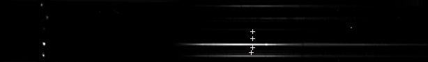
One the raw images of a 10 images sequence of HR Del, Cataclysmic variable. 120 sec individual exposure |

One of the raw offset images and the resulting offset once added |

one of the raw dark image. The dark images are acquired at an exposure duration equal or close to the star images to optimize the thermal dark subtraction process. and the resulting dark image once combined and offest substracted. |

Combined sum of the sequence, after offset and dark removal and registered with the l_register command of IRIS. The registration requires the selection of an absorption (or emission in this case) line feature on one of image of the sequence. The computation shift the all set of images considering the intensity profile selected, searching the center of gravity of the line and computing the shift for every images. It then recompute each image of the sequence with the previoulsy computed shift. The next step is then to add all the images and normalized the sum to the max intensity to avoid saturation. An automatic IRIS panel can lead you through all the steps at once...
|

Another step is usually required to align the star spectrum with the x-axis of the image to then perform a correct binning when reducing to a spectral profile. Different geometric transformation are available in IRIS, depending of the geometric distorsion observed. Tilt: to just rotate the spectrum of a predefined angle Slant: to shift lines by lines the star spectrum to have straight lines Smile: to eliminate the "smile" distorsion some times observed due to optical distorsion in the spectrograph. In our case, only tilting correction was required. |
The spectrum of the dark sky is superimposed on the star spectrum. To remove it, a zone is selected above and below the star spectrum and a column by column mean value of the sky zone is subtracted on all the image, including the star spectrum. Doing this removes the sky spectrum lines from the star spectrum. Several type of sky spectrum removal is available in IRIS, with different type of mean computing: single value, value per column, linear interpolation (l_sky3) to remove possible gradient as well. |
Once all the previous processing have been applied, I usually crop the image to keep only the star spectrum surrounded by dark sky, with no other visible object spectra before saving it for later processing and binning into Visual Spec |
| Spectral calibration |
|
To move from the image into a spectral profile, it is required to bin along the colum axis all the relevant intensity of the star spectrum. Two options are possibles: Automatic Binning
Visual spec applies a signal to noise criteria and pick only the lines which have an average intensity which maximize the signal to noise ratio of the mean profile. Manual Binning
The choice beetween the two is quite tricky and it's more or less by trying the two that one can be decided. If the spectrum is not well focalized, showing some chromatism the manual method gives a better result. |
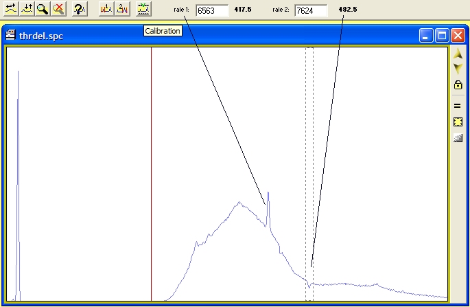
| The next step is to calibrate the spectrum regarding wavelength. In this spectrograph design, no calibration lamp was used. So the calibration used the lines of the star spectrum itself. In this case, no radial velocity can be computed later on.
The most used lines for linear calibration are the atmospheric line feature and one of Balmer line.
Final calibration in wavelength done, and spectrum cropped to show the relevant spectral zone. |
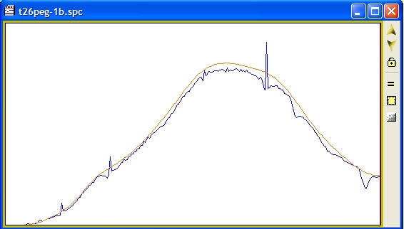
| The next step is to compute the spectral response of the system for the night. A standard star is used for this purpose, acquired in the same conditions (binning, grating, spectral domain) then the rest of the spectra. (or another reference spectrum shall be taken). Correctly pre-processed and calibrated as all the others spectra, the profile is then compare to the theoretical spectrum of the Visual Spec library from Pickles Atlas. The reference star is usually choosen not to close to the horizon (to minimize extinction effect) and of spectral type close to Vega like A0V. If the object spectrum is close to a solar type spectrum, as for comet of asteroids, it is better to pick a G-type star. Avoid I-III luminosity classes as emission lines can polluted the spectrum.
Reference star 26 Peg, of Spectral type A2V, with its theoretical spectral profile displayed. |
| The reference star spectrum is divided by the theoretical spectrum.
Below, the resulting division of the raw profile of the reference star by its theoritical spectral profile. Artefacts are due to spectral lines which have to be removed in the next step.
A strong smoothing process is then applied to remove the star lines and only the overall continuum variation is kept as the response curve. This profile is saved as the night response curve to be used to correct all the spectra and restore the "theoritical" flux variation.
Smooting operation by setting points where no lines are and applying a spline smoothing function.
In orange, the resulting final overall continuum response curve from the 26 Peg reference star. To perform an absolute flux calibration, the reference star shall have be picked from the Visual Spec response list (18 stars). Those 18 stars have their continuum calibrated in flux and by knowing the overall exposure time of the observations, the spectra can be corrected with this absolute response. In this case, the reference star shall be at the same elevation of the object studied or an extinction correction shall be also applied. |
| Once the response curve established for the all night, for each star spectrum the profile shall be divided by the response profile.
In green, the HR del spectrum, once the raw one in blue has been divided by the response of the above profile from the reference star 26 peg. |
The resulting spectrum can then be normalized, setting at 1 a pre-defined continuum zone, free of any lines. Arbitrarely, this zone has been set beetween 5200 and 5220 angströms in this processing. |
| At this point, Line Equivalent Width can be computed, but once the continuum is recalibrated to one on each side the line. This show the LEQ value for the emission H-alpha line.
|
![]()
![]()


 The user defines a zone around the spectrum, which includes all the star spectrum and almost no dark sky.