ISIS
Version
5
Guide
for process LISA spectra
1. Pupose
This guide provides an introduction to the use of ISIS (version 5 and above) in the context of LISA spectrograph spectra processing. We consider in the following that you have a basic knowledge on the use of software: setting initial configuration, viewing an image and a spectral profile, comparison of two profiles, etc.. For this, it is important to have read in advance the help page devoted to Lhires III and realized concretely proposed treatment, even if you do not use in practice this instrument. The Lhires page provides indeed a fast learning base fast to the fundamental principles of ISIS and with a sufficiently general pupose. See here.
We will deal in this guide as a processing demonstration (step by step) of a series of spectra of the symbiotic star CI Cyg (V=10,5 - see here for more info about the object). Vega spectra are used for calibration.
First we have to calculate the parameters calibration and spectral response instrumental Based on an observation of the bright star Vega made the same night.
Procedure for change ISIS langage interface.
2. Configure ISIS
You must first download the raw data that accompany this guide. It is strongly recommended to perform the processings at the same time you are reading this - you will progress very quickly in this way, being confronted with a real situation. Download the file:
Unzip the file (size 10.2 MB) into a directory of your choice. This will be your working directory for the observation session in question. For my part, I chose as directory
C: \ NUIT_20120914
Indeed, the data were acquired on the night of September 14 to 15, 2012. Verify that CALIB subdirectory is also created.
The observation was made with LISA spectrograph mounted at the rear of a Celestron 8. A focal reducer Baader (Alen Gee) passing the initial F/10 optical beam initial to about F/6.5 at the entrance of the spectrograph. The slit is 23 microns wide. The camera used for spectra acquisition is the model Atik460EX. The acquisition itself is performed by using very efficient sofware AualeLA. I use a binning 2x2 mode for the detector. The resulting virtual pixel size is 9.08 microns x 9.08 microns. The observatory it semi-urban with a strong light polution produced by high pressure sodium lamps.
Note: the format of raw images that are provided for this demonstration was cut vertically for a reasonable sized ZIP file. Of course, original scale is preserved. Also in order to limit the volume of data to be downloaded, the number of images in the sequence has been significantly reduced. The number of raw images of Vega was reduced to 3 when I actually acquired 16. For CI Cyg, I propose only the first 4 frames of a sequence original which actually contains 14. The idea is not the actual performance in the final result, but you learn good mothods to use ISIS.
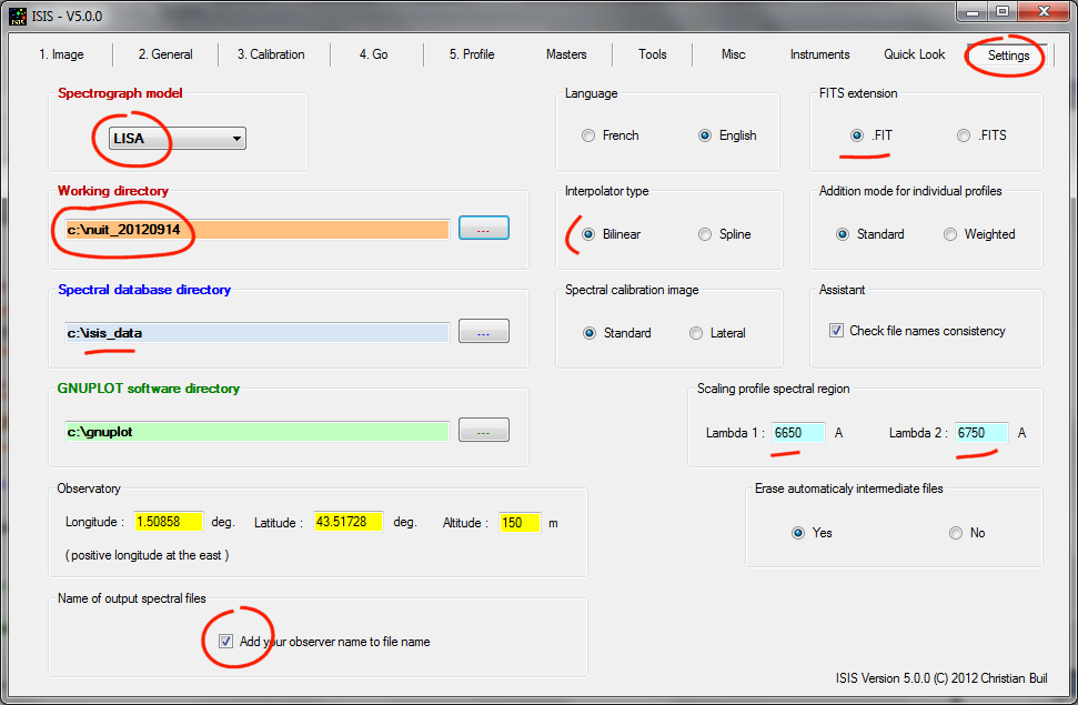
In the "Settings" tab, select the type of spectrograph used: here is the model LISA of course.
Specify the working directory: C: \ NUIT_20120914
Set a region in the observed spectra for scaling profiles. Choose valid valid for the spectral analysis (i.e. observed). Selecting a region in the red range from 6650 A to 6750 A (part of the spectrum free od intense spectral lines).
Check "Bilinear" for the type of interpolation (a precaution related to risk of processing artefact if you the "Spline" interpolator with LISA data).
Finally, select the option for add your observer name result files name (so that you identify the first glance if you distribute your results of observation).
Here the appearance of the "Configuration" tab at this stage:
3. Calibration
The same night as CI Cyg acquisition, a quick sequence of Vega star spectra was conducted to evaluate the dispersion equation of LISA spectrograph and instrumental response.
Note: the instrumental response in the sense used here also includes the atmospheric transmission. The star Vega was chosen because it is close to our target (CI Cyg), hence small difference in air mass.
The star Vega is not ideal for what we do now, especially find the instrumental response. It is an object too bright. The exposure time is only 0.1 second to avoid the risk of saturation. The star displacement due to seeing can cause errors in the continuum, which are not averaged because of the short exposure time. I alleviated the problem by performing 16 successive images of Vega, and average effect by addition of individual spectra (a task for ISIS!). For reasons of volume data, only the first 3 images in this sequence are available in the present distribution.
Ideally, to find the instrumental response, targeting hot stars (type A or B) with magnitude typically 4-6. Do not follow my bad example with Vega!
Display the first image of the sequence Vega (image files are named vega-1, vega-2, vega-3):

Go to the next step (number 2), click "General" button.
The "General" tab open automatically and ISIS complete a certain number of pre-filled fields, including the number of images in the sequence (3 images):

Because of the suffixes defined and respect of a strick protocol of nomination files during acquisition (very useful and important to make life easier), the "Calibration" field is also pre-filled.
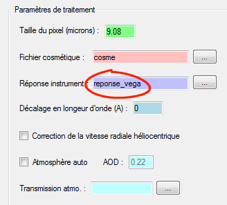
Do not forget to enter the pixel size of your detector (with binning), and include a description of your instrument, your observatory and yourself.
Also confirm the "Optimal binning" option.
For the rest, it is assumed that the master images offset signal and thermal (named here "dark") are calculated (note that the detector temperature is -5 ° C, it sees that the name given to files). A cosmetic file (cosme.lst) identifies deviants points. The method to achieve these master images under ISIS is described here.
Turning now to step 3 by opening the "Calibration" tab:

The contents of the first frame of the sequence is automatically displayed. ISIS also calculates the Y coordinate of the middle of the spectrum (because the "Auto" checkbox is selected). The software
find Y = 134. Note that we also choose to display the reticle for a visual control of slected pertinence for binning areas and measurement of the sky background.
We will first perform the spectral calibration. A wizard is available for it. To activate it, click the "Calibration assistant":

The aspect of (spectral) calibration assistant:

The first operation is to calculate an average image from the input images of the sequence. The goal here is to compute (vega-1 + vega-2 + vega-3) / 3.
Normally, the fields "Generic Name" and "Number of images" in the section "Calculation mean image..." are prefilled. If this is not the case, enter info in the "Root name" and "Object Name" in the "Definition automaticaly file names" section and click "Go".
Enter a name for the mean image.. We choose: mean (not very original - eventually you always use the same name, because it is here only an intremediate image file for present calculation only. Click "Go":

The result output section informs you precisely about the calculations. Now you have an image a mean images of three raw Vega spectra images in the working directory.
Note that the name "average" was copied automatically in the next section "Spectral Calibration with ...".
To find the calibration coefficients (or dispersion equation), we will use a mixed technique, mixing the contents of the reference star (here the mean Vega spectrum) and the content of the image of internal LISA neon lamp acquired immediately after Vega sequence, and named "vega_neon-1". Incidentally, we have not yet had the opportunity to view this image calibration!
The spectrum of the star is used to find the dispersion parameters in blue, neon spectrum is used to find these parameters in the red. For initialize the calculation, your only action is to identify the Halpha line in the Vega spectrum, and then perform a double-click on it with the mouse pointer (do not close the calibration assistant):

The result is automatically reported in the wizard:

Coordinates found for the Halpha line are X = 969, Y = 134 (you could set these values from the keyboard if it is more convenient for you). The accuracy assessment does not need to be very high. Do not take yourself too head to position the pointer when you double click. A difference of 3 or 4 pixels is quite tolerated.
Everything is right to perform the spectral calibration. Simply click on the "Go" button:

Square error spectral calibration (RMS, Root Mean Square) is 0.22 A. This is a small error and with the typical procedure used (spectral sampling is of 3.5 pixels, so, the typical calibration error is nearly 1/10 the size of a pixel).
We want to push the calibration as far as possible in the blue. If you check the "UV Calibration" ISIS selects stellar lines located further to the blue, in the ultraviolet region of the spectrum. This gives additional validity to coefficients for calibrate ultraviolet part of the spectrum. You can use this option because the Vega spectrum has a high signal to noise ratio and the setting is such that the blue part of the spectrum is quite sharp. Most often this option leads to an average degradation on the whole spectrum. Here is the result in this case:

The RMS error is now 0.24 A, which is still quite acceptable. We may retain choice.
For curiosity, you can view the calibration coefficients of the polynomial computed (up to order 4):

Note that these coefficients are retained even if you exit the program.
Close the window of the spectral calibration wizard ("Close" button).
Note: calibration image vega_neon-1 is of great importance, but it is used in the background by ISIS. You can of course display this image if you are curious:

Note the position of the line crresponding to wavelength 5945 A. The position of the mouse pointer indicates the horizontal coordinate X = 797. Open now the "Calibration" tab and look carefully fields automatically filled by our calibration wizard:

ISIS has rightly selected himself in neon line ar 5945 A and evaluated automatically associated X correctly. Note also that ISIS find automatically tilt angle and slant angle of the spectrum. Much less operation to perform manually.
We will now proceed to search the instrumental spectral response. As always, it is the most delicate operation!
Open the wizard "Response assistant" (click on the button):

First calculate flat-field image. This is done using an image sequence of internal LISA tungsten lamp LISA spectrograph, made just after Vega sequence Vega. Quite logically, the images of this sequence are called: vega_tung-1, vega_tung-2-3 vega_tung ... Do not hesitate to make a large number of images of this type (especially for reduce noise in the blue part of the spectrum). I take18 elementary flat-field images with a peak intensity reaching about 55,000 digital encoders unit. Here, we have only first 5 images of this sequence for reasons of space when downloading:

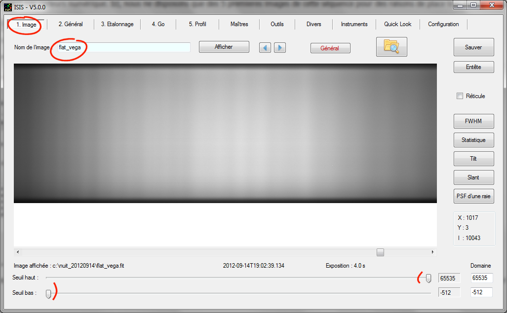
After clicking "Go" ISIS give details of the operations and produce image flat_vega.fit in the working directory (this is the name chosen by us).
Here, the final flat-field image calculated:
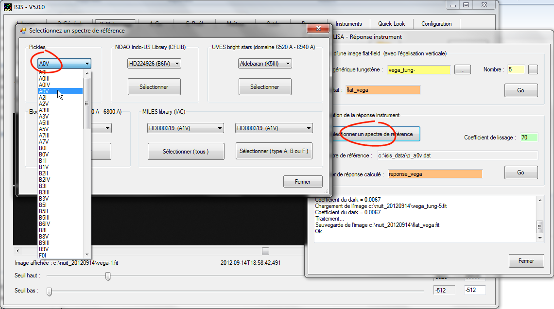
Vega is a A0V type star. We will divide the observed spectrum of the star by the theoretical A0V spectrum. First we isolate a reference spectrum from ISIS database. From the wizard "Instrument response", click "Select a reference spectrum." In the box dialog that opens, select spectrum a Pickles type A0V spectra. Spectra based on Pickles are theoretical spectra of stars classified according to their type spectral. Confirm your choice by clicking on the "Select" button:
ISIS recalls specral type of selected reference (more precisely, the file name in the database):
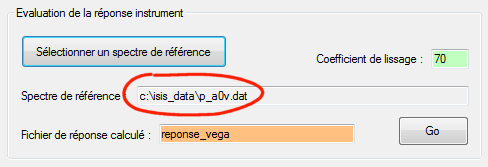
We will now proceed to the division of the observed Vega spectrum by a synthetic A0V type star. First enter the name of the file that will contain the result of the division. This is the final instrumental response file name. Logically we give the name: reponse_vega. Implied a spectral response calculated from a spectrum of the star Vega. Provide a value in the "smoothing factor". This amount may seem esoteric at this stage, but you'll quickly understand. Give for the mopment the value 70. Then click "Go":

The software performs a large number of operations. In particular, a complete processing of Vega sequence, but ISIS mask you these things. It calculates the famous ratio and displayed directly it the "Profile" tab, which opens automatically as well.
ISIS still carries a smoothing of the ratio (star observed) / (theoretical star). The strength of smoothing is adjusted by the coefficient that we have set to 70, arbitrarily. But how do you know the right value? This is the most difficult and it takes a bit of work. Take a test. Change the value of the coefficient, adopte value 10, then remade "Go":

The appearance of the instrumental response has completely changed (note the appearance of a high-frequency noise). Do the opposite, using a high value for the coefficient, eg 200:

This time the smoothing is much larger, but also the appearance of the spectral response curve is changed again. So where is the truth? You probably understood, we will have to proceed by trial and error, blindly if you want. Something that is more difficult to explain than to do. This is why I suggest you perform the processing at the same time as you read this tutorial.
To help you, the best way is to compare the response curve which the unsmoothed ratio for a certain coefficient.
Do not close the assistant window "Instrument response", set in a corner of the screen. From the "Profile" tab, click on the "Compare" button in the vertical tool list.
Complete the dialog box as shown below, then click on the "Compare" button:

What's going on? First we have provided the name of the spectrum to compare "@@". It is an intremediate spectral profile (which is not intended to be preserved), stored in the working directory, which is the ratio between the observed star and theoretical spectrum (before smoothing). When you press the "Compare" button, ISIS simultaneously displays:
- Blue, smooth response that we have calculated;
- Red, unsmoothed response (the contents of @@ file).
The goal is quite simple: the blue curve follows the red curve closely, but without the noise appears and residue artifacts (trace of telluric lines
in particular) because this details not reflected in the true instrumental response. This is arbitrary, but unfortunately we do not have another means really reasonable.

This is a little better with the coefficient of 60 adopted in this test. However, the blue curve does not return the curve in the spectral response visible near 4200 A, which is quite typical spectral response for the spectrograph LISA. The problem is actually the internal tungsten lamp spectrograph that displays abrupt changes in intensity in the blue. The phenomenon is more or less pronounced depending on the model. In my case, it is particularly strong, so that the curve
response is extremely distorted, which is never a good situation. This complicates our task. The responsable of situation is not ISIS but LISA spectrograph!
Restitution of the rapid curve change at 4200 A is a good criterion for determining the value of smoothing coefficient. Test the value 20 now:

It's not bad, but simultaneously the smoothed curve fit residues of telluric lines. Even a small effort to refine compromise with the value 25:

This is good, your "reponse_vega" now contains a correct instrumental response. With practice, gradually as you learn how to use LISA/ISIS association, you will result in faster and with greater assurance in a few moments.
Close the "Comparison spectrum" and the assistant "Instrumental response" dialogs.
Take a look at the "General" tab:
ISIS has filled in for you the "Inst. responsivity" field. All is OK for full process Vega spectrum. Open "Go" tab and press the "Go" button:

It'll just look at the result, for example, clicking on "Display Profile" from "Go" tab. The "Profile" tab opens automatically with the spectral profile on the screen:

To be convinced that the spectrum is correctly processed, compare with the spectrum of a star A0V Pickles. Use the "Compare" and will load directly in the spectrum ISIS database (note the spectrum is in .dat format):

Blue curve, the observed spectrum, red curve, spectrum spectrum (less spectrally resolved). The overlay is really excellent, including the extreme blue. One can even guess the limit of the Balmer series in the ultraviolet (this is particularly due to the good quantum efficiency CCD Sony on camera Atik460EX). The restitution of continuum is also very satisfactory.
4. Processing CI Cyg spectrum
Most of the work has been done on Vega spectrum. Following processing becomes very simple (be careful though, if you observe spectra at angular heights very different it will surely necessary to recompute specral response by choosing a reference star near your target). Let us CI Cyg.
Will show the first spectrum of the series:
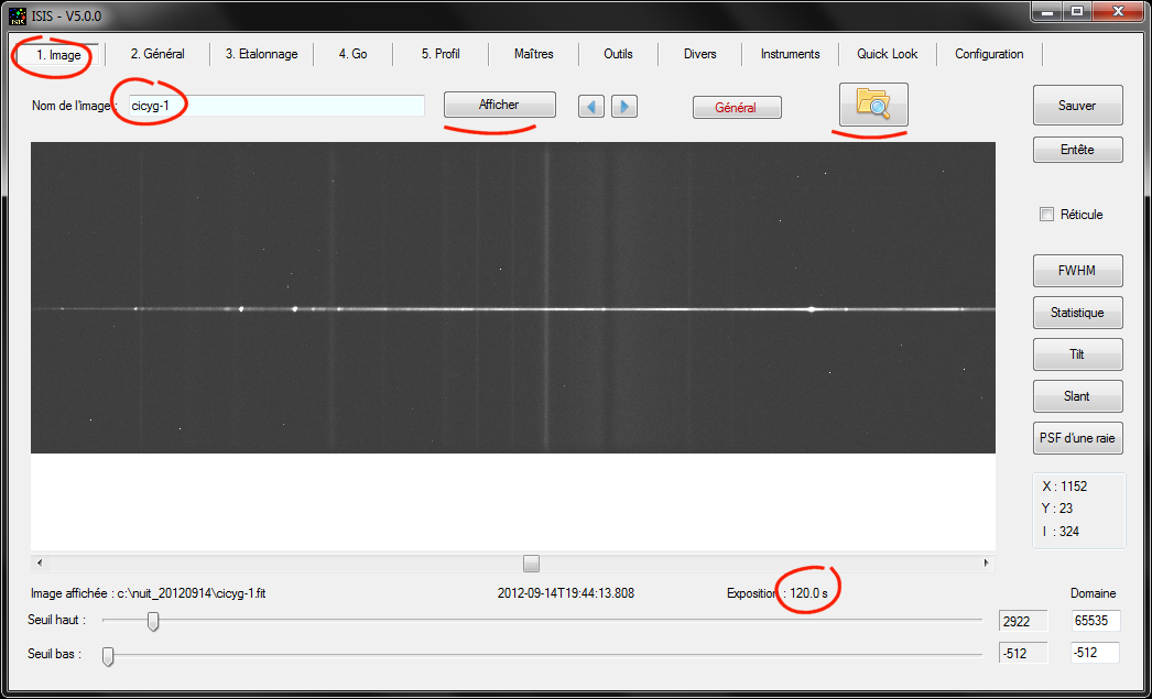
The spectrum is spectacular: a cool star with numerous intense emission liens. Note the exposure time of 120 seconds, always reminded in the tab. Note also presence of urban pollution spectrum in the background.
Click on "General" button. The "General" appears:

Enter the name of the object. We choose "CI Cyg."
The rest is prefilled, including the name of the calibration image: cicyg_neon-1. This is important. This is because we have a good protocol during acquisition had careful during acquisition (coherent names for object and calibration images).
Open "Calibration" tab.

The spectrum produced by the LISA spectrograph is always sharp. So, you can reduce the width of the binning zone. This limits the risk of cosmic rays presence.
Go to "Go" tab, then click "Go" button:

And display the result:

You can crop the spectrum for the area corresponding to a signal to noise ratio reasonably strong:

Finally, save the result of cropped profile. Use the same name as output of principal processing:

As a control purpose, do not hesitate to display 2D images:

Here, the CI Cyg processed 2D (image) spectrum:

Geometric corrections are made (eg the spectrum is perfectly horizontal). Note also that the lines of the sky background also disappeared.
5. About specral calibration
When you use the spectral calibration assistant for LISA, ISIS suppose is configured for use of dispersion equation already calculated. You can see that this mode is automatiquely selected by opening the "General" tab (section "Spectral calibration"):
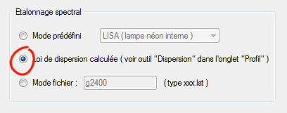
Systematically, if the preset mode is selected, ISIS will seek the calibration coefficients in the dialog box "Compute spectral dispersion", a tool that is
opened from the "Profile" tab and the "Dispersion" button:

Note that it is possible to change "by hand" coefficients values. They are also kept from one session to the next.
There is one other option for LISA calibration, using a preset mode for this special spectrograph:
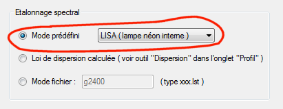
If you choose this option, ISIS performs processing using only the spectrum of neon lamp - you do not need to observe a reference type A or B star, at least for spectral calibration (spectral response, is something else). Consequently, it is unnecessary to use the spectral calibration wizard, you skip a step. The procedure is simpler, but less accurate. To realize this, load into memory calculation parameters for Vega spectrum via its XML file (see Lhires III tutorial). Change only the calibration mode through the preset mode LISA. Go directly to the "Go" tab, and start the processing. Finally, examine the spectrum calculated and compare with A0V Pickles:

The result is not catastrophic, but still significantly worse than the mixed method (star + neon). This is the difference between a medium qualty pectrum and a high quality spectrum.
Note: for the preset mode works must, expose well the neon lamp for reduce noise in the blue, even saturating red. An exposure time of 10 to 30 seconds for the neon lamp is usually sufficient for this specific pupose.