7 : Processing of high resolution spectra in detail
We have previously described some principles of operation of specINTI and we have quickly shown an example of processing. Here we go into more detail on the constitution of the observation and configuration files, which are at the heart of the principle of the application, while delivering tips for the acquisition and exploitation of spectra, more precisely in the perspective of high spectral resolution spectrography. As support, we keep the "starex213" session, already used previously.
We remind you that all the data attached to the example can be downloaded as a ZIP archive by clicking on this link: starex213.zip
7.1 : How to properly complete the observation file?
To facilitate the learning process, we will only describe at the beginning the processing of a single object, the spectra of the bright star Altair, centered on the famous red H-alpha line of hydrogen. Our archive proposes 6 images of the raw spectrum of this object with the names altair-1, altair- 2, ...., altair-6. These images were acquired in sequence, one after the other. The individual exposure time is 45 seconds.
Note: these are image files in FITS format, but the ".fits" extension is deliberately ignored because specINTI will add it for you.
Another associated image file is present, discrete, the "altair_neon-1" file. This is the image of the spectrum of the light emitted by a neon gas spectral lamp (precisely, a discharge lamp containing neon gas, as is sometimes found in electrical installations). We'll see its usefulness later.
Let's open the "Observations" tab in the specINTI Editor interface.
First, you must indicate in which folder the images to be processed are located, i.e. the path of the working directory. We have already talked about this in the previous section: at the very top of the tab, click on the "Browse" button, then from the dialog box that opens, locate your working folder, then select it.
Then specify the plain name of the object to be processed in the "Object list" field, here "Altair" (upper or lower case, it does not matter). This name is not chosen at random: it reminds the generic name of the raw images and is recognized by SIMBAD.
At this point, specINTI Editor offers an automation mechanism. Click on the "Auto" button. The software then fills in many fields for you. It automatically finds the generic name of your raw files ("altair-"), the number of images in the sequence (6), the presence of the spectral calibration image "altair_neon-1" (the software also understands that there is only one such image available).
Tip: notice the use of the "-" between the generic name and the index number. This is to avoid confusing the latter with the catalog number. As already mentioned, it is highly recommended to use this dash when building a list of objects (even if there is only one object in this list).
Note: for the automation mechanism to work, specINTI Editor must know the type of separator between the generic name and the index number (the "postfix"). Given the way we name files (including spectral calibration files), you should set the "postfix" as follows (these settings are retained when you exit the program, it is not necessary to set them the next time you use specINTI Editor):
It is also necessary to take care of the offset, dark and flat-field images, necessary for good pre-processing of the raw images. We are here in the classic of astronomical image processing.
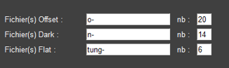
There are two ways to do this with specINTI. The first is to provide the generic name of the corresponding image sequences and the number of images (this number is found automatically by clicking on the well named "Auto" button). Let's suppose that you have 20 raw images of the offset signal, named o-1, o-2, ... o-20, 14 raw images of the dark signal (long exposures in the dark), named n-1, n-2, ..., n-14, and finally 6 flat-field images of a continuous spectrum lamp (we will see later how to acquire these), named tung-1, tung-2, ..., tung-6. In this case, enter the following elements in the dedicated area of the tab "Observations":
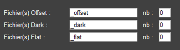
The second way is that after the first processing with the generic name of the pre-processing images, provided as above, specINTI automatically writes images with reserved names in the working folder: _offset, _dark, _flat. These are the processed master images of the offset, dark and flat-field signal, respectively. Processed means that for example the 20 offset images have been averaged, the offset signal has been subtracted from the 14 dark images to get a true thermal signal map for the temperature and exposure time used, etc. So in a next processing you can perfectly write (which will be a bit faster in terms of calculation) :
Note that the number of images provided is 0 because _offset, _dark and _flat are not generic sequence names, but simple file names.
It is still possible to mix pre-calculated master images with raw calibration images in list form. This is the situation for our observation "starex213" where we propose to use the pre-calculated images _offset and _dark, and a raw sequence of 6 flat-field images having the generic name "tung-", which gives in the end :
Note: a question is often asked about the exposure time to choose for dark (or black) images. Should we use the same exposure time as for the images of astronomical targets? Fortunately, the answer is no! In our case, the exposure time for each of our 14 elementary dark images is 900 seconds (1/4 hour). If you have to process a spectrum exposed for 60 seconds, there is absolutely no point in calculating a dark image generated from elementary images exposed for 60 seconds, because specINTI adjusts the basic master dark image of 900 seconds to simulate a dark image of 60 seconds. Moral: make dark images with a time at least as long as the longest exposure time used on the targets, and that's it (never process a spectrum exposed for 600 seconds with a "dark" exposed for 60 seconds, because then the noise becomes very strong). The very important point is that the temperature of the detector must always be the same, for example here -12°C (if necessary, to remember, you can name your "dark": n900_12-1, n900_12-2, ..., a good trick to find your way, because some acquisition software do not write the temperature of the sensor in the FITS header).
To complete the editing of the "Observations" tab, remember to give a name to the observation file. By clicking on the "Save" button, specINTI Editor saves your observation file in the current working folder (mandatory). It is a file respecting the YAML architecture, in text format. You are free for the name. Here we have chosen "obs_altair" (with the understanding that we are processing an observation of the star Altair). By double-clicking on the name of this same file (or another one), which then appears in the list on the right, you display its contents in the "Observations" tab. This is very useful to find the way you have processed old data.
7.2 : How to display the image of a spectrum?
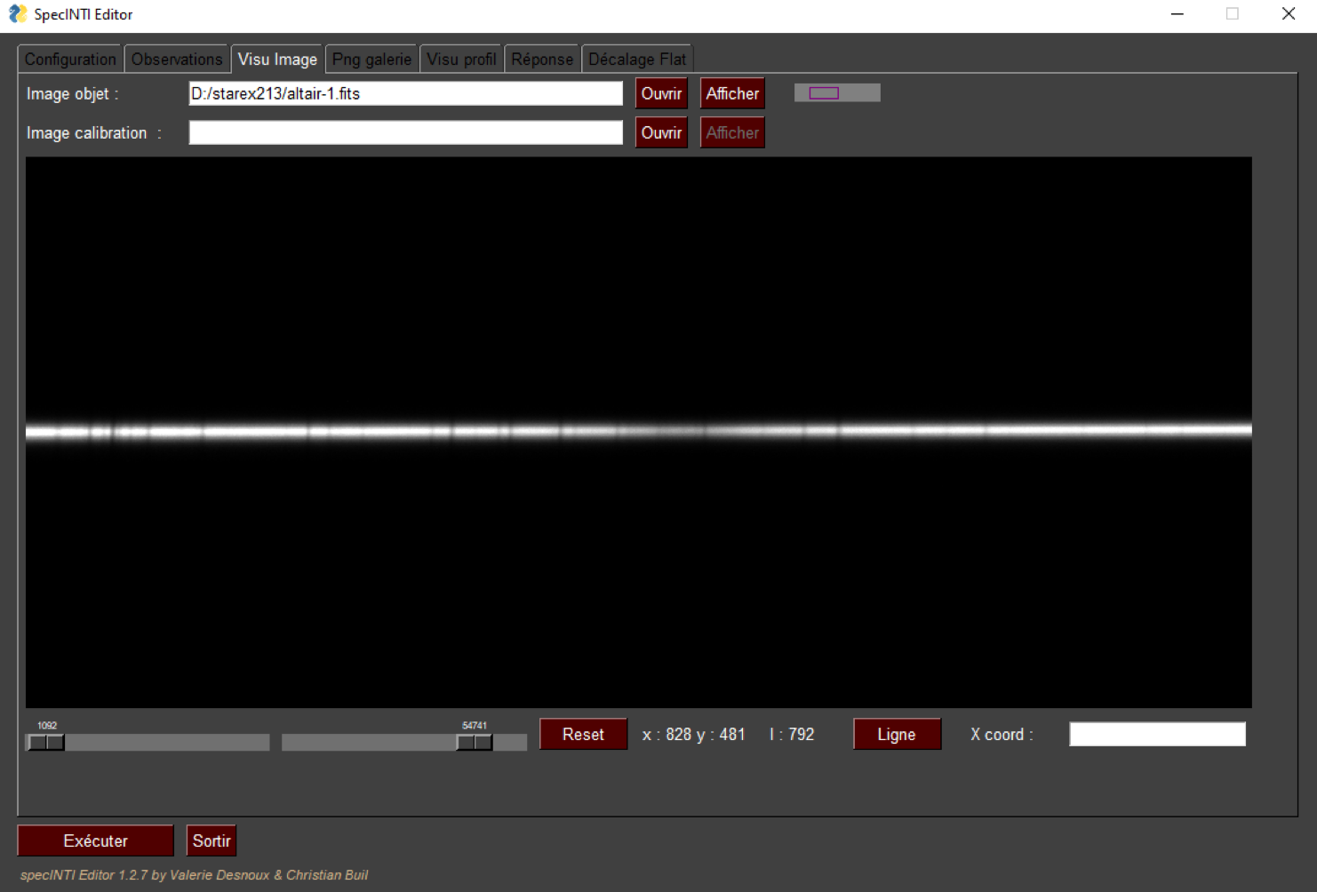
You may be curious to know what a raw image of the Altair star spectrum looks like? It is very simple. Go to the "Visu Image" tab, click on the "Open" button, select the file altair-1.fits (for example) in the working directory, and the spectrum image is displayed immediately:
Here you can see only an excerpt from the captured image. To move around within the image, drag with the left mouse button held down. Learn to use the horizontal sliders at the bottom of the tab, which allow you to adjust the contrast and brightness. To find out the intensity of a point in the image, position the mouse pointer, then left-click.
The global image itself shows only a portion of the spectrum of the star Altair, in the red part, approximately centered on the H-alpha line. It is typical of a high-resolution spectrum acquired with the Star'Ex spectrograph, or any other spectrograph of the same category: the actual spectrum of the star is the thin horizontal line. The H-alpha line is the large absorption indentation that can be seen a little on the left of the image. This unusual width for this type of star comes from the fact that the star rotates very quickly around its axis, which produces a very significant Doppler-Fizeau broadening of the hydrogen line and all other stellar lines in the spectrum of this object. The fine lines are telluric lines, i.e. lines that appear when the light of the star crosses the thin layer of our Earth's atmosphere. The lines in question come from the absorption by the H2O molecules (water vapor in the atmosphere) - we will return to this.
Note: the H-alpha line is not centered on the portion of spectrum captured. This is deliberate, to be able to simultaneously observe a helium line which is located further in the red, on the right side of the image.
It is important to note that we have exploited during the acquisition of the image only a fraction of the detection area offered by the Sony IMX533 sensor, which has 3008x3008 pixels (ZWO ASI533MM camera). The image acquired, and that you display on the screen, is only 3008 pixels wide and 651 pixels high. At the time of acquisition, with the software used (Prism), we made sure to keep only the part of the image considered as useful, the ROI (from the English "Region Of Interest"). The spectrum being a line, it is logical to keep only a band around the trace. This cropping avoids unnecessary saturation of the hard disk, accelerates calculations and gives a more pleasant display. Working on the ROI is a very important habit in stellar spectrography.
In addition, the acquisition was performed in 1x1 binning. Again, this is an important consideration when working with a CMOS sensor. Of course, a 2x2 binning, for example, reduces the size of the images, but it is a destructive operation, which eliminates very useful information to exploit the optical image of the spectrum. You can't go back after a 2x2 binning, the damage is done. You must not work with CMOS sensors other than in 1X1 binning if you want to get the best out of your images (we will come back to this later).
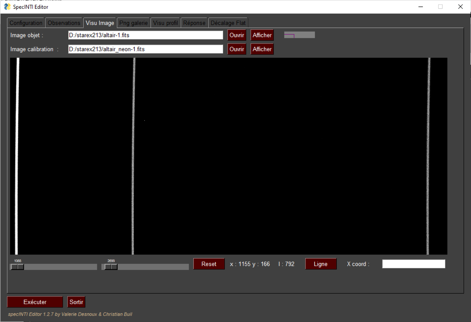
You can display other images of course, altair-2.fits, _offset.fits, tung-4.fits, ... The image altair_neon-1.fits (you can use the second display field, useful for image comparisons) is particularly instructive too:
We see the emission lines produced by the spectral calibration lamp - the thin, approximately vertical lines. These lines are associated with a very narrow spectral range and perfectly identified in wavelength. We speak of "monochromatic" lines, while the spectrum of our star is "polychromatic" (it contains several wavelengths, or colors).
If you are a little attentive, you will notice that these lines are slightly curved, which must be taken into account during processing. This curvature is called a "smile" in English (a "smile" in French). It comes from a variable incidence of light rays on the diffraction grating of the spectrograph depending on whether the rays come from the center of the slit or the edge. This results in a slight variation of the dispersive power of the grating depending on the height considered on the slit, hence the curvature. This effect is clearly visible with a grating of 2400 lines/mm, but very attenuated with a grating of 300 lines/mm, for example, so that it goes unnoticed.
We explain in the following section how this reference spectrum of neon was actually obtained.
7.3: The acquisition of the spectral reference source
We have just glimpsed the aspect of the spectrum of the neon lamp, which will be one of the elements of the wavelength calibration of our spectra (the process of associating a wavelength to each pixel along the spectral axis of the image).
The "traditional" method to obtain such a "monochromatic" line spectrum consists in placing just in front of the spectrograph (between the telescope and the spectrograph) a kind of light box in which is housed the emission line spectral source. A servomechanism, often controlled by the acquisition computer, allows either to let the light of the star being observed pass freely, or to send the light of the standard source to the slit. Depending on the case, the acquisition of the spectrum of the star, or the spectrum of the standard lamp. This assembly at the front of the spectrograph is often called "bonnette".
We note first that it is not possible, in the simple form described, to simultaneously acquire the spectrum of the star and the spectrum of the reference spectra. This time shift is a source of calibration error if the instrument bends under its own weight over time or if a temperature variation occurs (this is called "thermo-elastic" deformation). At the very least, it is necessary to ensure that the time between the acquisitions on the sky and the calibration acquisitions is short, even if it means alternating them ideally, but it is tedious.
One of the disadvantages of the traditional method is that it represents a point of fragility as soon as a mechanism is implemented. It also generates extra weight at the end of the telescope. There is also a financial surcharge. Finally, it is generally not easy to house in a small volume an optical device that simulates the aperture ratio of the telescope when the light of the standard lamp is injected (ideal to avoid some calibration bias due to residual optical aberrations of the spectrograph).
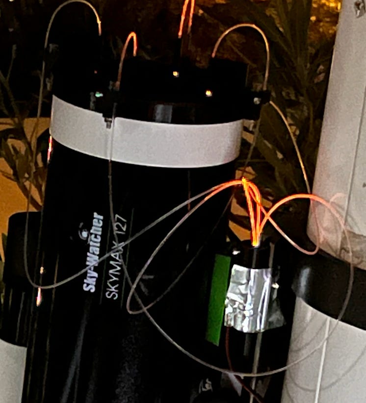
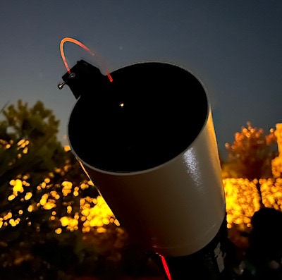
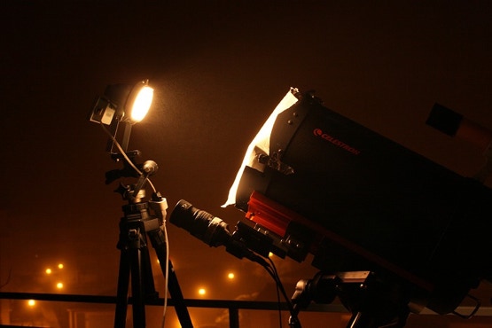
Our technical approach is very different in the example provided, in break with the habits. It consists in placing at the front of the telescope tube or telescope, one or more lamps producing the spectrum of reference lines, as shown in the images below:
The flux can also be conducted to the entrance of the telescope via one or more optical fibers (plastic fibers are suitable, with a large diameter, with a possible scissor cut, and a very low cost, see for example here). It is the fiber technique that we used for the acquisition of the spectra that illustrate this demonstration:
We can make a small light box, as in the example opposite, which includes the start of the fibers and integrates a simple neon nightlight lamp with E10 base, powered by 220V but beware, through a 12V to 220V converter for safety reasons. Never 110/220V direct on a telescope!
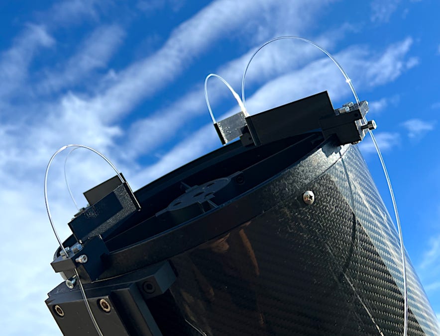
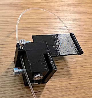
As an example, here's how a 1.5 mm CHINLY plastic fiber is mounted on the front of a 100 mm-diameter telescope using a two-part 3D-printed assembly (click hereto download the corresponding STLs). Note that the fiber is positioned at the center of the lens, minimizing spectral calibration bias.
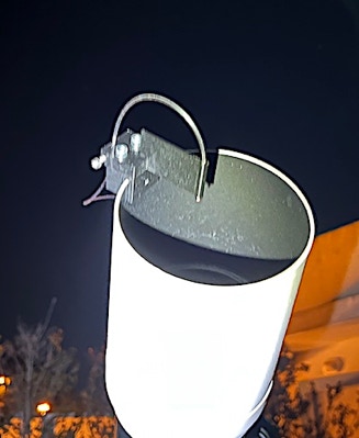
Hereafter the assembly to be adopted to exploit in full safety a discharge night light (neon or any other gas). We use a 220V-12V power supply, then a common 12V->220V converter. We also give the reference of the neon lamp with E10 base recommended because well luminous (LG234 230V), under the reference 582852 at the supplier Conrad.
The better the illumination is distributed over the entrance pupil of the telescope or refractor, the better the result will be, but one illumination point can already be sufficient. If the illumination is punctual, it is recommended that the points be located at 0.7 times the radius of the telescope (or telescope) starting from the center and in the extension of the long axis of the slit. Contrary to what one might think, this illumination in the pupil is very little intrusive. If you do the ratio of surfaces, you will see that its impact is negligible compared to that caused by the central obstruction of the telescope. The support parts are easy to make in 3D printing. A simple neon light, with E10 base, powered on 220V (via a 12V->220V converter) is quite suitable.
The interest of this mode of injection of the light of the standard source is that it is a static system, without mechanism, light, being able to be left in residence, and of a very low cost (it can be tinkered in one day). We also work as close as possible to the optical path followed by the light of the stars. In addition, the lamp can be lit intermittently, via a computer command for example, but also permanently while observing the celestial targets, in order to practice a continuous calibration, efficient and which will be described in section 6.
7.4: The acquisition of the "flat-field" source
Let's look at how to acquire the flat-field images, tung-1, tung-2..., used in this demonstration. Here again, we are breaking with our usual habits.
Traditionally, the flat-field is realized thanks to a light box placed just in front of the entrance slit of the spectrograph, but with the same shortcomings as underlined for the spectral calibration (difficulties to represent the telescope aperture, complexity, clutter). It is sometimes more convenient to illuminate the entrance of the telescope in a uniform way, as shown in these views, because the calibration flux follows the same path as the stars, and the focal plane is more bare.
For intermediate size telescopes (say, up to 300 mm diameter), this technique is viable and produces good results. But it also raises difficulties. It requires an intense source to have a correct flat-field signal, with a minimum of noise (high signal to noise ratio, especially in the blue). The choice of the nature of the lamp is limited: halogen spotlights heat up quickly, LED panels have a very chaotic intensity curve depending on the wavelength (not very favorable to treat the case of a spectrum realized in low resolution). The environment is also copiously lit. Finally, as the telescope grows, the device becomes heavy and the operation consumes time.
In the end, we choose a much lighter and simpler technique. We will work on the table, in a very local way, by momentarily decoupling the spectrograph from the telescope. Only the entrance of the spectrograph, of small size, is then illuminated with a white lamp to obtain the flat-field. Here is an arrangement:
The lamp is an incandescent filament bulb containing a halogen gas (krypton) which gives a very white light. We note at the entrance of the 31.75 mm slider the presence of a small diaphragm simulating the aperture ratio of the telescope, covered with a light diffuser (simple sheet of tracing paper). The whole is made in 3D printing. The unfortunate thing is that it is becoming difficult to find tungsten filament lamps because of the advent of LED lighting (LEDs are a calamity for spectrography, and astronomy in general, contrary to what we can hear here and there. Of course, the electrical efficiency of a LED is high, but the quality of the light emitted in urban lighting is very poor for the sight, because in general too much blue, because the whole visible spectrum is polluted (unlike what we get with a high-pressure sodium lamp), because the control circuits are expensive and often fail, because it is a solution of ease often used wrongly ... In short, this mode of lighting is much less ecological than it is said to be, whereas the good old sodium lamps for urban lighting were a blessing because of the quality of the light emitted, in all respects.
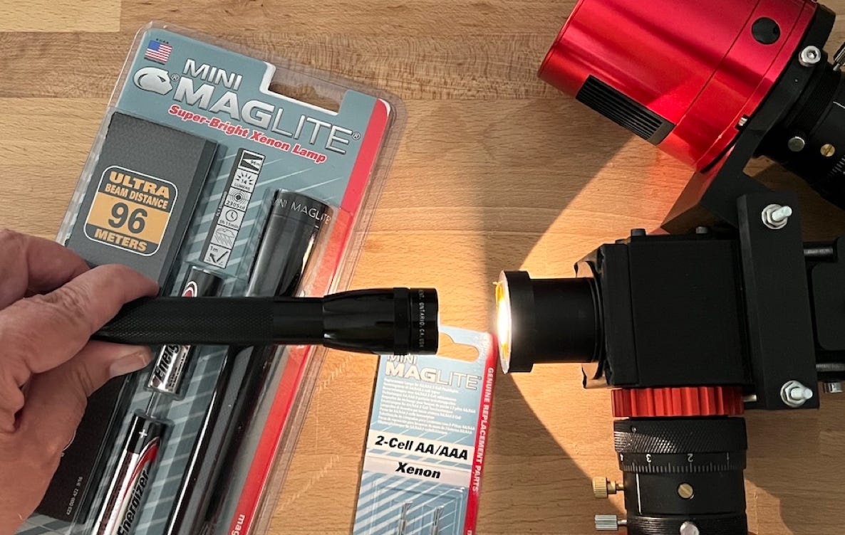
An alternative, which is very simple, is to use as a flat-field source, a MAGLinte flashlight, which still produces models with incandescent filament of tungsten to xenon halide:
What diameter should be given to the diaphragm? Suppose that the distance between the entrance of the slit and the plane of the diaphragm is 76 mm. If we want to simulate a telescope aperture of f/8 (F/D=8), then the diameter of the hole must be 76 / 8 = 9.5 mm. Remember to cover the diaphragm with a piece of tracing paper to make the illumination even on the surface of the diaphragm.
The realization of flat-field images is therefore distinct from night observation. It can be done when you want (during the day for example), without stress and by dedicating the night to the observation of the targets (avoid to disturb or to shake the spectrograph too much between the moment you observe and the moment you take the flat-field). The exposure time for our tung-1, tung-2,... images is only 2.6 seconds (of course you have to avoid saturating the detector). This time is so short, that we do not hesitate to multiply the number of flat-field images for a minimal noise in particular in the blue of the spectrum. In this demonstration, there are 6 tungsten images, but in fact, we have acquired 30 - only the first 6 of the series being delivered here).
7.5 : The configuration file in detail
Open the " Configuration " tab from specINTI Editor, and double click in the list on the right, on the title conf_starex2400_mode0_demo0.yaml. This is a configuration file already present in the "_configuration" subfolder of the software installation directory:
The text that appears in the window on the left is a set of parameters describing your instrument configuration and how you want to process the spectra. The parts of the text that appear in gray are comments, to help you find your way around. Let's look at the contents of this configuration file, as we propose it here. Here is the complete listing:
The file is composed of several lines, which are as many parameters, except the comment lines (they start with the character "#". But good news, for a given instrumental configuration (your own spectrograph in plain language) and if you don't move, the value of these parameters doesn't change, except at the margin. A configuration file as presented is thus a kind of frame or canvas, on which you will graft some adjustments. But of course, you must know the meaning of the parameters.
Note first that the order in which they appear has no effect on the processing, so you can group these parameters by category for better readability. Some parameters are mandatory, while others are optional.
As far as syntax is concerned, you have to be strict. First, there is the parameter title, followed by the character ":" (no space). Then comes a space (only one!), then the value of the parameter, which can be a number, a character string, or a list of values (which is put between square brackets).
Let's take two examples of parameters:
calib_mode: 2
norm_wave: [6400, 6420]
The first one, "calib_mode", is here assigned the value 2. This determines how specINTI will go about calibrating your wavelength spectra.
The "norm_wave" parameter is associated with a list of two values (in square brackets), setting the wavelength range within which specINTI will normalize the final spectrum to unity.
There is only one parameter per line, and the name of a parameter is unique in the configuration file (no way to define twice the parameter "norm_wave" for example in the same configuration file).
Important: be careful, if you make a mistake in the syntax of a parameter, it will not be taken into account in the application and there will be no error message (the way to check that the operations are done correctly is to examine the output in the console which gives a lot of details).
Now let's review our configuration file. The first parameter encountered in the listing is called "working_path". This is a required parameter. The value is the path to the working folder.
Tip: when you edit the observation file and save it, the value of the "working_path" parameter is automatically updated in the configuration file. This saves time.
The next parameter, "batch_name", also mandatory, has for value the name of the observation file describing the data to process. In the example "obs_altair" (the .yaml extension is not indicated). You can write in lower case or upper case.
Tip: the value of this parameter is automatically changed when you save the observation file, just like the "working_path" parameter.
The "calib_mode" parameter is mandatory. It specifies the type of spectral calibration performed during processing. Several strategies are possible, described in section 10 of this manual. They are numbered 0, 1, 2, 3, 4. Here the mode used is number 0, in a way the basic mode for easy spectrography, and ideal for high spectral resolution.
In order for specINTI to work in this mode 0, it must be provided with the name of at least one image containing an emission line spectrum from a reference lamp, in addition to the name of the images to be reduced. You have recognized the file "altair_neon-1", reported in the observation file. We arrange for specINTI to automatically find the lines in this spectrum so that it makes the link between the pixel numbers and the wavelength. This link is found via a mathematical method called "least squares", from which the terms of a polynomial function are fitted as best as possible. This function, a polynomial of a certain degree, links a pixel number to a wavelength. It is also sometimes called "dispersion polynomial" (spectral).
The presence of the optional parameter "auto_calib" forces specINTI to automatically find the spectral lines in the image file "altair_neon-1", to identify them by their wavelengths (from an internal catalog), to measure to a fraction of pixels the position of these lines in the image, and finally to establish a dispersion polynomial, which is then applied to the sequence of objects processed. The "auto_calib" parameter, when present in the configuration file, triggers a complex and powerful process (but this only applies to the H-alpha line region and for high-resolution spectrography (R > 10000).
In the observed spectral region, we can identify 5 usable neon lines, shown below in superposition to a star spectrum:
You will easily find them in the image "altair_neon-1". However, examine the appearance of the line at 6717 A on the right. It appears more blurred than the previous line at 6678 A. We are confronted here with the optical limits of the Star'Ex spectrograph in the chosen configuration. Above the wavelength 6700 A, we admit that the optical aberrations are too high to exploit the spectrum correctly (too much "blur" in the image). We will therefore exclude the line located at 6717 A for the calculation of the dispersion polynomial. This explains the values given to the parameter "auto_calib", a list of two numbers in square brackets:
auto_calib: [6500, 6700]
This instructs spectINTI to find the calibration lines only between the wavelengths 6500 A and 6700 A. The potentially problematic line is thus eliminated from the calculation. In the end, the calibration is performed from n=4 lines, taking into account this choice.
The maximum degree of the calibration polynomial being equal to n-1, we can not use a polynomial of degree greater than 3. This is a good thing, because in high resolution, a polynomial of degree 2 already provides a sufficient accuracy.
To indicate to specINTI that the dispersion polynomial to be evaluated is of degree 2, we must add the parameter "poly_order", with the value 2, as it should be:
poly_order: 2
Tip: if for some reason the automatic search for calibration lines fails (you will get a message in the output console), you can remove the "auto_calib" parameter from the configuration file, and exchange it with two parameters, "line_pos" and "wavelength", through which you provide respectively the (approximate) position of the selected emission lines and their precise wavelengths from a catalog. The result is the same as with "auto_calib":
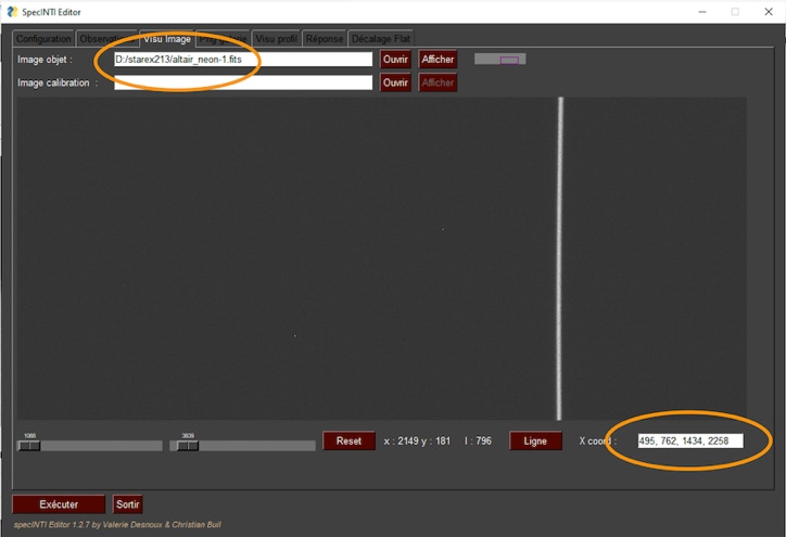
Another little trick. Display the image of the neon spectrum, click on the lines successively from the left, while holding down the "Allt" key. The horizontal position values in pixels are then found in the "X coord" field. You just have to copy these values and then paste them as is as an argument to the "line_pos" parameter.
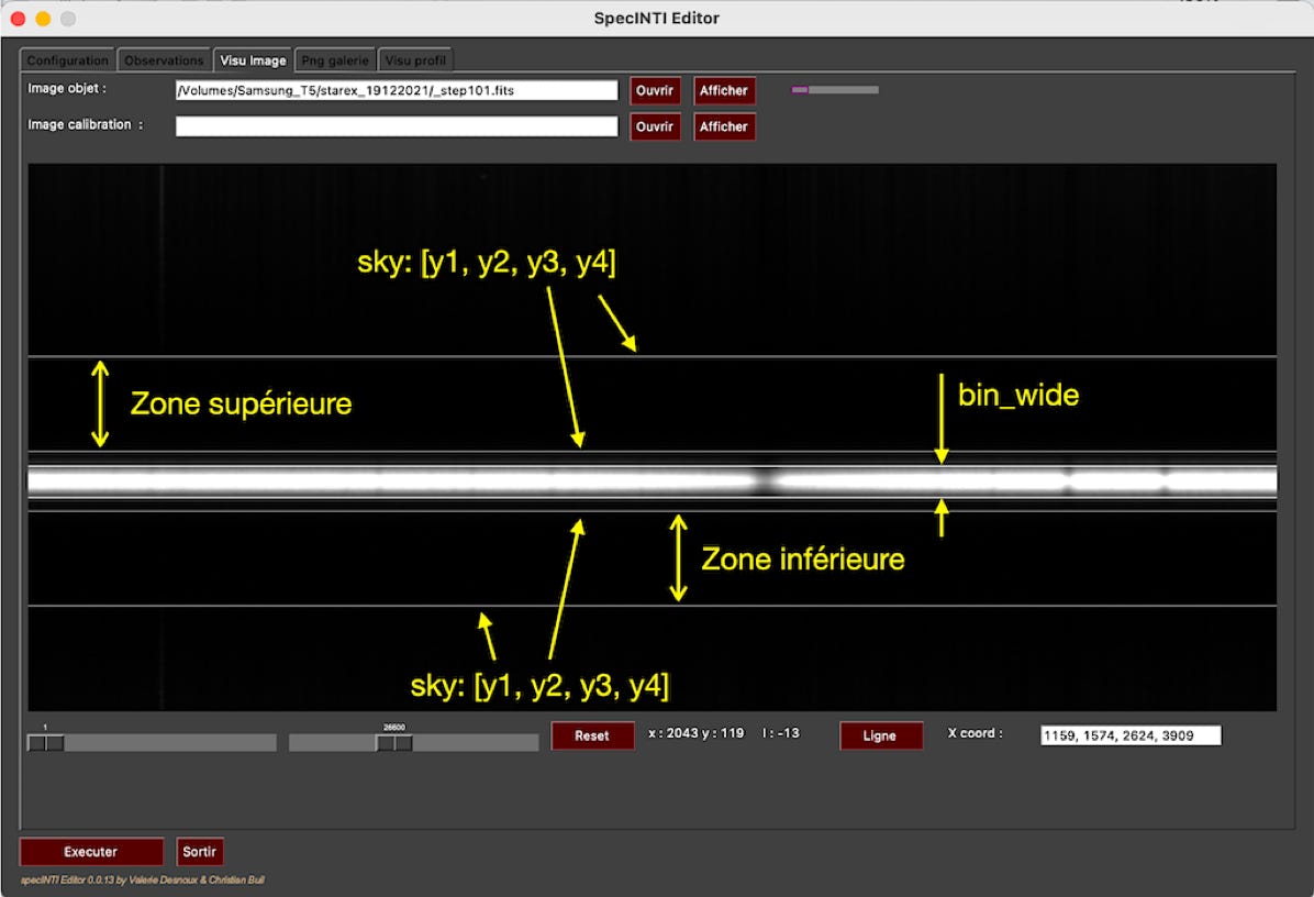
The value of the "bin_size" parameter defines a vertical width around the 2D spectrum trace within which specINTI will perform a summation of the image intensities, column by column to build the spectral profile point by point:
A good strategy to find a correct value for the "bin_size" parameter is to make this width cover 99% of the effective signal (along the vertical axis of the image). But the value of "bin_size" should not be so excessive (except when using an optimal profile extraction algorithm - a possibility described in section 5.6), otherwise the noise will increase unnecessarily while the signal does not. Here the binning area is chosen to be 22 pixels high.
It is important, for the spectral binning operation to achieve a good result, to first remove the signal of the sky background, which is a parasite. It is the role of the "sky" parameter to indicate to specINTI how it should proceed. The purpose of this removal is to keep only the signal of the star in the spectral profile. Even if the sky intensity is often low in spectrography, because of the presence of a narrow slit at the entrance of the spectrograph, the operation should not be neglected (light pollution, for example, is visible as discrete lines or diffuse bands that can clash with the true spectrum of the star if nothing is done). The work consists in removing from the binning area, column after column, the signal found on both sides of the spectrum trace. This measurement of the background is done in two regions located on each side of the trace, whose widths and positions are defined as values of the parameter "sky". The positions in pixels are relative to the vertical coordinate of the trace:
In the example, the sky background evaluation area is between -20 and -120 pixels from the bottom of the trace, and between +20 and +120 pixels from the top of the trace, as shown in the diagram above. An evaluation area height of the sky background of 80 to 150 pixels is considered satisfactory as a general rule. Two algorithms are proposed for this operation, which can remove more or less efficiently accidental signals in the sky background calculation area (cosmic ray trace, for example). The method used depends on the optional parameter "sky_mode", see section 5.8. But as this parameter is not present in the configuration file, the simplest technique is used, and also the fastest, and sufficient in this case.
Next we find the "smile_radius" parameter:
# --------------------------------------
# Smile radius
# --------------------------------------
smile_radius: -24000
The phenomenon of "smile", which amounts to a curvature of the lines, has already been mentioned previously. This curvature of the lines is problematic when performing binning, because in its presence, we agglomerate intensities corresponding to different wavelengths. This effect induces a loss of spectral resolution and alters the shape of the lines. It is therefore important before anything else to modify the geometry of the spectrum by calculation so that the lines are vertical after calculation:
The value of the "smile_radius" parameter is the radius of curvature of the smille in pixels, here evaluated at r = -24000 pixels. The sign indicates the orientation of the curvature. From this information, specINTI generates an inverse smille effect of r = +24000 to compensate for the apparent smile produced by the optics, and thus result in straight lines. A problem is that the current version of specINTI does not allow a direct numerical evaluation of the radius of curvature of the smile effect. It is necessary to find this value by trial and error, in order to obtain geometrically rectified lines that are vertical and straight.
There are several ways to find the value of the radius of curvature, by a simple visual observation. Let's use the simplest one, which will also allow us to understand how to act in the configuration file and interpret the intermediate calculation results.
First, deliberately assign an erroneous result to the "smile_radius" parameter, for example a radius of curvature of R = -4000, by modifying the current value in the configuration file :
smile_radius: -4000
Let's make another change to the configuration file. At the bottom of the configuration file you will find the parameter :
check_mode: 0
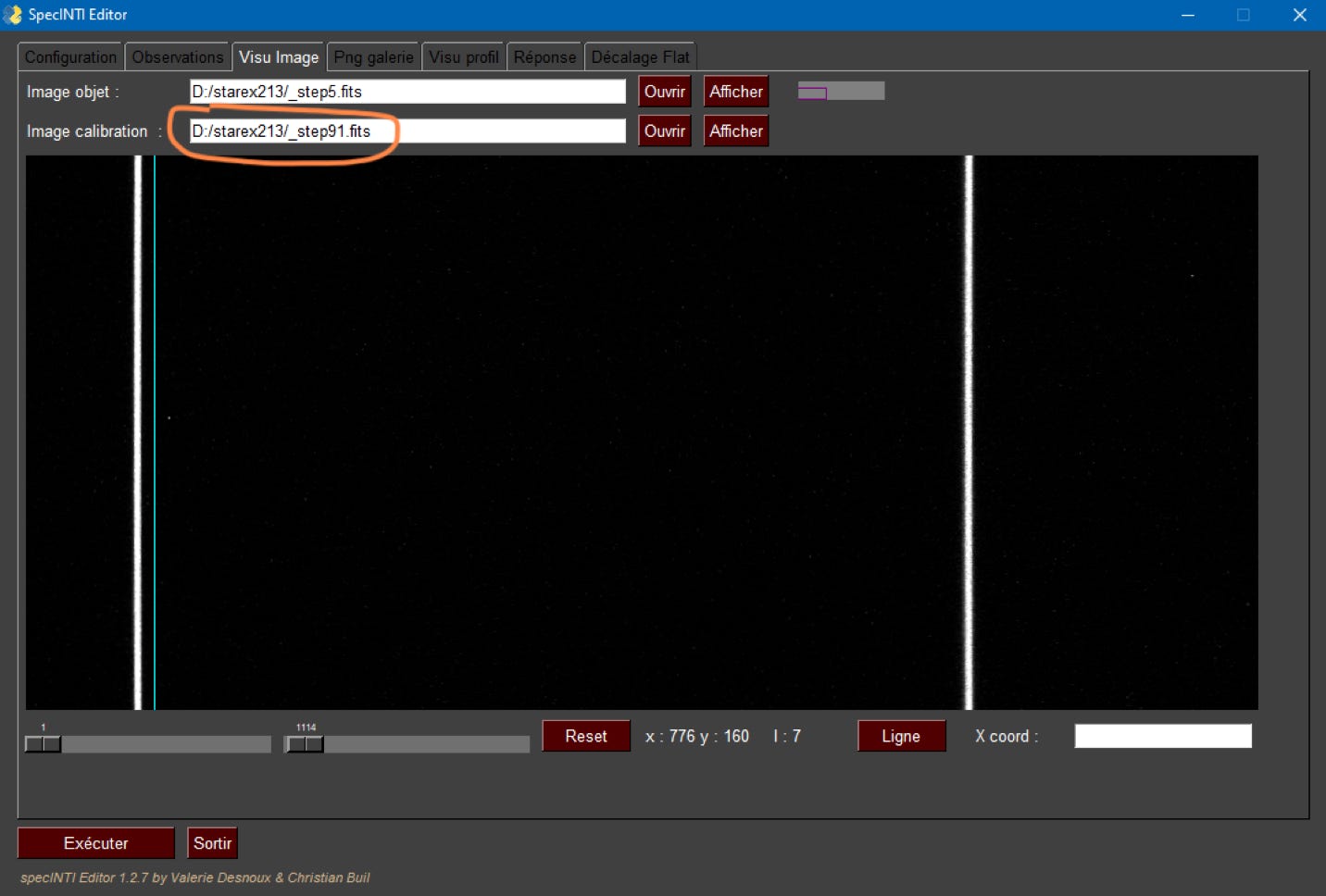
This parameter, which is optional, controls the level of detail of the information delivered to the console and to your disk when the program is run. If the value of "check_mode" is 0, we are in an option that provides very condensed information (this is also the default value, if the optional "check_mode" parameter is not present in the configuration file). Set the value of "check_mode" to 1 to get a maximum of information about the program flow in the console. When this value is used, the software writes a number of profile and image files to the working directory, which, when properly interpreted, will help to detect a processing anomaly. We have artificially produced such an anomaly with the smile radius. Set the value of "check_mode" to 1, and launch the processing by clicking on "Run". You will notice that the "log" in the console is much larger than usual. Then open the "Image view" tab and display successively images called "_spec5.fits" and "_sptep91.fits", the famous intermediate data. The image "_step5" shows the appearance of the spectrum of the standard lamp before geometric rectification:
Tip: you can display a vertical cyan line in the image, as in the document above, which helps to gauge the value of the smile. To make this line appear at a given point in the image, click on the point in question (left click), while holding down the "Crtl" key on the keyboard.
Let's now display the image "_step91". This shows the image of the neon spectrum after geometrical "correction", when the parameter "smille_radius" is defined in the configuration file:
The smile is strongly overcorrected because of the wrong value provided with "smile_radius". Now do :
smile_radius: -24000
then restart the program:
The lines and the guide reticle are now well parallel, we have found a satisfactory value for the "smile_radius" parameter (there is a good tolerance, a value of R=-20000 will not make much difference, for example).
Tip: if you want to speed up the iterative process, temporarily indicate in the "Observations" tab that you have only one image of the Altair star spectrum, instead of 6.
The "xlimit" parameter delimits an interval in pixels in the image of the spectrum of the stars within which specINTI performs a number of automatic geometric calculations (locating the Y coordinate of the trace (vertical) in each image of a sequence, inclination of the trace (also called "tilt" angle, ....). The chosen area should enclose a fairly well visible and uniform part of the spectrum trace. In the example, the area is generously wide, delimited on the left by X=300, on the right by X=2200 (this is very flexible)
The (optional) parameter "norm_wave" defines an interval in wavelength within which the software will calculate an average (thus, in the spectral profile), then perform a normalization of the entire spectrum so that in the interval in question, the average intensity is equal to 1 after the operation. You are free to choose the normalization area. Here the spectral range is 6640 A - 6660 A, chosen because it is free of intense stellar lines.
The (optional) parameter "crop_wave" is again a spectral interval, but this time it defines a clipping zone of the spectrum in order to eliminate the parts considered useless (too much affected by noise or insufficient spectral resolution, for example). Here, the final spectral profile will be limited by the wavelengths 6500 A - 6700 A.
Defining the optional parameter "planck" in the configuration file forces specINTI to correct the signal found in the spectrum of the flat-field images (here tung-1, tung-2, tung-3...) in order to take into account the color temperature of the incandescent lamp used. This information allows to obtain a spectral profile of the stars closer to the expected one. The distribution of the spectral signal from a lamp such as a MAGlite (see section 5.4) is assimilated to that produced by a black body, and the value of the parameter is the temperature of this body in Kelvin. In the demonstration, we choose a temperature of 2900 K, a little bit passe partout and close to the real temperature for the type of lamp used.
The parameters "longitude", "latitude" and "altitude" provide the coordinates of the observation location (the angles in decimal degrees, the positive longitude east of Greenwitch, and the altitude in meters). These parameters are optional, but it is recommended to define them in the configuration file. These coordinates will be found in the FITS header of the processed profile.
With the parameters "site", "inst" and "observer", you can indicate the name of your observation site (observatory), the type of instrument with which the current configuration file is associated, and the name of the observer. All these elements will also be found in the header of the FITS spectrum files. It is recommended that you define them as they are your signature of sorts.
Tip: you can add the optional "file_extension" parameter, which specifies the type of FITS file header, anywhere in the configuration file. The default value is zero, and corresponds to the extension ".fits". If you use the value 1, the extension is ".fit". Example,
file_extension: 1
Of course you have the possibility to save the configuration file you just edited. Use the line "Configuration file to save" at the bottom of the tab. The location of the backup is necessarily the subdirectory "_configuration" of the specINTI Editor installation directory. For example:
conf_RC10_starex2400_VIS.ymal
The "conf_" at the beginning indicates that it is a configuration file. Then comes a description of the instrument that is specific to you. Here the type of telescope, a 10 inch Ritchey-Chretien, then a brief description of the state of the spectrograph (here a 2400 t/mm grating on a StarEx spectrograph optimized for the visible). You can build up a library of configuration files in this way if you operate several pieces of equipment. At this stage, for the demo, we use the corresponding YAML parameter file « conf_starex2400_mode0_demo0.yaml » (see « _configuration » sub-directory).
7.6 : How to reduce noise
The reduction of the measurement noise is always an objective. The challenge is for example to obtain a readable spectrum (with a signal-to-noise ratio of at least 5) for objects of the lowest possible brightness, knowing that the value of the signal is limited by the duration of the exposure, which always finds a limit (patience, length of the night, the need to optimize the number of objects observed, etc).
The specINTI software offers several possibilities, in the form of optional parameters, which can be used separately or together. Here are the main ones.
The first of these parameters is called "sky_mode". It concerns the way the sky background is calculated and then subtracted from the raw data to extract the true profile of the star without radiometric bias (see the "sky" parameter). If the value of the parameter is 0 (default value), the sky background is found column after column of the image by averaging the median signal found on both sides of the trace. If the value is 1, an interpolation algorithm based on Legendre polynomials evaluates the sky background signal. Generally speaking, this last algorithm estimates the sky background better, which reduces noise and some artifacts, but the calculation time is significantly longer.
The parameter "extract_mode", when defined, implies that the software performs an "optimal" extraction of the spectral profile during the binning phase of the image (agglomeration) to achieve the spectral profile. To do this, the "extract_mode" parameter must be set to 1. More precisely, specINTI implements here an algorithm known as "Hornes algorithm", widely used for the reduction of astronomical spectra. The idea is to apply a weighting when adding the signal column after column, depending on the signal and the noise. Thus, the points located far from the center of the trace along the spatial axis (vertical) have their noise reduced, because they also correspond to a signal of low value, with a small final contribution. Moreover, the algorithm is of the iterative type, with the aim of eliminating the trace of cosmic rays, likely to produce false detections in the spectrum.
A complication is that the Hornes algorithm requires that the gain of the camera (e-/ADU) and its readout noise (in e-) be known, respectively transmitted to the software through the parameters "gain" and "noise". We show in section 11.3 how to find these values experimentally if they are not already known. For example, with an ASI533MM camera from ZWO operated at a manufacturer's gain of 150 (15 dB), we have: gain = 0.083 electron/ADU and noise = 1.3 electron (with an ASI183MM camera used at a gain of 200, we have g = 0.041 e-/ADU and noise = 1.8 e-)
The efficiency of the algorithm is only really perceptible when dealing with signals of very low intensity compared to the noise (typically a signal to noise ratio lower than 20). In other situations, you can return to a more basic algorithm (simple arithmetic summation in the binning width), either by not defining "extract_mode", or by giving the parameter the value 0 (in this case the "gain" and "noise" parameters are of no use).
The parameter "kernel_size", when set, or when it has a value other than 0, makes the program perform a non-linear filtering of the median type on all the images of the sequence. When the parameter is set to 3, it means that the calculation kernel is a square of 3x3 pixels. A filtering on a kernel of 5 pixels side is also possible, the value of the parameter being then not 3, but 5. In its basic form, this filter is quite destructive: it removes very well the "salt and pepper" noise (or RTS noise, also called "percutional"), but also, very often, real details of the image. It is not recommended to use the "kernel_size" parameter in this way. On the other hand, if you give the parameter a negative value, -3 or -5, it is still a median filtering that applies, but based on an algorithm that filters the noise well, while preserving the details. This is a filtering mode that we sometimes call CMED (for CmosMEDian). However the use, even with negative values, of this type of filter is possible ideally only if the width at half maximum (FWHM) of the resolution element is greater than 4 with the -3 filter and greater than 6 with the -5 filter. This is why the CMOS data are imperatively acquired in binning 1x1 on the telescope. Here the FWHM is 5.5 pixels (see the "log" in the console), so we can use the optimized median filter -3. The idea is that the frequency of the details that we want to erase (noise) is significantly higher than the optical frequency of the spectrograph. The result is always quite spectacular with CMOS sensors, affected by a generally high RTS noise (this is not the case with the old CCD sensors, for which the CMED does not have to be applied, but simultaneously, CMOS sensor + CMED gives in the end a noise lower than that offered by the CCD cameras)
The "sigma_gauss" parameter imposes a Gaussian type filtering on the raw images (as well as on the images of the calibration lamp). This filtering softens the appearance of the images and it is therefore quickly possible to reduce the power of resolution. For the case treated, the value of the filtering will be 1.0 (standard deviation of the filter, with a filtering all the more accentuated as the value is strong). The application of this filter reduces the resolving power from R=13000 to R=12000, which is considered reasonable, because the noise decreases faster than the resolution (again a question of sampling the spectrum images). Do some tests by monitoring the result in the log.
If you want to use all these noise reduction techniques in our demonstration, add the following lines somewhere in the configuration file (see modified parameters file is in the distribution, under the name "conf2400_mode0_demo1.yaml"):
Here is the profile of the Altair star after application of these noise remedies (compare before and after filtering):
Before filtering.
After filtering.
7.7 : The accuracy of the spectral calibration
At the end of the reduction work, is the spectral calibration really fair, really accurate, and by how much? A large number of events can deteriorate the quality of this calibration. The most frequent problem is the time that elapses between the moment when we take the "science" images and the moment when we take the calibration images. This time lapse is conducive to distortions of the instrument, sometimes tiny, but with a noticeable effect in the final spectrum. Another classic cause of error is the difference in the path of light rays coming from the "science" and calibration sources (the errors are then of the systematic type).
It is therefore always good to be suspicious and to check, from time to time, that everything is going as well as expected. specINTI Editor offers a tool to perform this check, especially adapted to spectra with high spectral resolution around the H-alpha line, which is precisely our situation. We use a natural spectrum, which always leaves a trace in the spectra of our stars (unless we observe in very high mountains with very dry air): the telluric lines of water vapor (H2O). This chemical element of our atmosphere produces a spectrum of fine lines in absorption, with perfectly known wavelengths. It is precisely the comparison between the observed wavelengths and the wavelengths of the line catalog that will allow us to evaluate the quality of the spectral calibration.
Display the reduced spectral profile of Altair (via the tab "Visu profile", then click on the button "Check atmo" located in the lower part of the tab. specINTI Editor draws marks at the expected location of the main H2O lines, as well as the deviation (in A) between the measured position and the catalog. You can zoom in with the magnifying glass to better examine the details:
We then realize that the telluric lines are shifted towards the blue of about -0.07 A. This deviation is quite small, 1/7 to 1/8 of the spectral sharpness delivered by Star'Ex, but still clearly perceptible with the implemented tool, that one should not hesitate to use. The defect can be explained by a thermo-elastic variation of the spectrograph between the moment when the spectra of the star are taken and the moment when the spectrum of the neon is captured (at the end of the observation session of the Altair star, whereas ideally it would be necessary to take a reference spectrum at the beginning of the sequence and another one at the end of the sequence, specINTI then taking care of making a kind of average if one has more than one calibration spectrum).
Once the spectral calibration error is known, it is easy to correct it by using the optional parameter "spectral_shift_wave", whose value is the negative of the spectral shift observed in angstroms (i.e. +0.07 A). Add this line in the configuration file, and run the processing again:
spectral_shift_wave: 0.07
The observed telluric lines are now almost perfectly aligned with their catalog positions
(the modified the corresponding YAML configuration file is « conf_starex2400_mode0_demo2.yaml » - see « goodies » section):
Often, the shift observed is a constant, from one target to another, and so the "spectral_shift_wave" parameter can remain in the configuration file. Note the existence of the "spectral_shift_vel" parameter whose value is this time a shift in velocity (km/s), which means that it is then possible to perform a rigorous Doppler-Fizeau shift over a wide spectral range (because the Doppler shift is not linear with the wavelength).
7.8 : Evaluation of the instrumental response
7.8.1 : The theory
Before reaching the telescope, the light of the observed star crosses the Earth's atmosphere, which has the effect of modifying its apparent spectrum compared to what it is in reality. Indeed, the atmosphere behaves like a colored filter that attenuates certain wavelengths more strongly than others. The absorption is on the one hand continuous (aerosol scattering, Rayleigh scattering, which gives its blue color to the daytime sky), ozone, and on the other hand, localized in the form of bands (H2O, O2) - this is the molecular absorption.
It is the continuous absorption induced by the atmosphere that is by far our main concern and that we must seek to erase.
The traditional method to rectify the continuous distortion of the spectrum by the atmosphere is to observe at a small angular distance from the star studied a star whose real spectrum is perfectly known (in tables, catalogs). The comparison between the apparent spectrum of this reference star (the observed one) and the spectrum in the catalog (real spectrum) allows to evaluate the impact of the atmosphere, then to correct it in the spectrum of the target under study. This technique gives good results, especially since it also partly corrects a subtle effect: atmospheric chromatism (the atmosphere refracts light rays according to their wavelengths, which affects the overall shape of the spectrum, especially in the blue and UV). Unfortunately, this "differential" technique is rather tedious (ideally, for each target made, one should take the spectrum of two objects that are not in the same field), and one does not always find well-placed reference stars. Moreover, in this situation, the ratio between the apparent spectrum and the real (catalog) spectrum of the star is often called "instrumental response", but this is a misnomer. Indeed, the shape of this response depends on the state of the atmosphere, while the latter has nothing to do with the instrument. What is called here "instrumental response" is a curve that varies according to whether we observe near the horizon or at the zenith, from one night to another. Obtaining this "pseudo-response" thus requires a substantial effort of observation, which wastes time and energy.
Our proposal here is very different since it aims to evaluate the "true" instrumental response, i.e. a constant for a given instrument, wherever one points in the sky and at any time. The effort is then focused on the estimation of the atmospheric transmission, especially its continuous part. It is your computer that will take care of this, calculating the result for you in a fraction of a second. We proceed in three steps:
(1) first we observe a so-called "reference" star, whose true spectrum is available in a catalog (spectrum as seen outside the atmosphere and corrected for all instrumental biases). In our demonstration, this reference star is none other than Altair. Indeed, a reference spectrum is available for this star. Start by downloading a database of spectra specially built by us from this link (ZIP archive): data_base.zip. Unzip it in a folder of your choice. You will find a large set of reference spectra, very useful for the following, and in particular an extract of the spectrum of the star Altair, obtained with the very powerful UVES spectrograph in high resolution which equips one of the VLT telescopes of ESO. It is considered reliable and available under the name "UVES_altair.FITS". Copy this file in your working directory. Here is the profile of this spectrum (see the source here):
(2) the apparent spectrum of Altair, such as we have reduced it at this stage with specINTI, is converted into a spectrum such as we could see it from space, by applying the inverse optical transmission of the atmosphere of the moment. Concretely, the operation is simple: we divide the apparent Altair spectrum by the evaluated atmospheric transmission. It is specINTI which takes care of the operation.
(3) after the division, we have the spectrum of the star only distorted from reality by the response of the instrument (optical transmission of the components, quantum efficiency of the detector, etc.). The evaluation of the "true" response is then trivial: it is the result of the division of the spectrum of Altair out of atmosphere by the catalog spectrum of this star.
The power of the method is that if you do the same operation with another reference star, and if you do not make an error in the evaluation of the atmospheric transmission, you will find the same result. A possible discrepancy may be a sign that the impact of the atmosphere has been incorrectly estimated or that there is a more subtle problem of atmospheric refraction (if possible, observe the stars at zenith to eliminate this effect).
The contributors to the true answer thus found have no reason to see their characteristics evolve over time. They are therefore constants. The instrumental response outside the atmosphere is also a constant by consequence. The moral is that the latter needs to be evaluated only once, and certainly not for each observed star. The time saving is significant and things become easier at night, when minutes are counted so few opportunities to observe.
In this section we describe the tools to find the spectral signal outside the atmosphere, as if we were in the vacuum of space.
specINTI proposes a tool to find the transmission of the atmosphere in the direction of the targeted sky, a result that depends at first order on two parameters:
(1) On the amount of aerosol present in the atmosphere, which opacifies it more or less to optical radiation. The measure is given by the AOD = Aerosol Optical Depth (see for example: https://earthobservatory.nasa.gov/global-maps/MODAL2_M_AER_OD). The higher the value of AOD, the more opaque the atmosphere is. The AOD is measured by ground or satellite surveys. But the simple observation of nature (horizontal transparency) already gives indications. Remember these values for the AOD: a very dry mountain air corresponds to an AOD of 0.02 and for a dry desert the AOD is 0.04. In France, the AOD is 0.07 in winter, 0.21 in summer, and on average over the year of 0.13. When the weather is very hot and stormy, the AOD can reach 0.50. For our observation, made in summer, near the sea, but not on a properly transparent night, we adopt the average value: AOD = 0.13.
(2) The angular height of the star with respect to the horizon line. specINTI automatically calculates this angle for you, but beware, it is imperative that the header of the FITS files contains the following keywords: DATE-OBS, CRVAL1 and CRVAL2. The last two correspond respectively to the right ascension and declination of the target star, with the values in decimal degrees.
7.8.2 : The calculation of the diffuse transmission of the atmosphere
In our scheme of evaluation of the true instrumental response, the cornerstone is the calculation of the diffuse atmospheric transmission under the conditions of the observation.
Let us specify that considering the way we acquired our spectrum during this starex213 session, by observing a small portion of the red spectrum of the star, the effect of the atmospheric transmission is discrete. The thing becomes more serious if we observe a more global set of the spectrum, and in particular its blue part (see section 7 of this documentation). However, let us play the game, and calculate the state of the atmosphere, even in the context of the observation of the star Altair in high spectral resolution around the H-alpha line.
specINTI integrates a fairly accurate atmospheric transmission model, which requires only one parameter to be activated and its associated value: the AOD (see above). Note that the specINTI atmospheric model includes aerosol scattering, Rayleigh scattering and absorption by high altitude ozone.
The estimated value of the AOD at the time of the observation is passed to specINTI through the "corr_atmo" parameter. For example:
# ---------------------------
# Atmospheric transmission correction
# ---------------------------
corr_atmo: 0.13
Not only does the software calculate the atmospheric transmission, but it also rectifies the spectra profiles so that they become as if they were seen "out of the atmosphere" (by the way, it is spectra corrected in this way that should normally be used for scientific analysis, the Earth's atmosphere being a parasitic element in the case).
For the calculation to be done, specINTI needs the angular height of the star with respect to the horizon line, and therefore needs to know the date of the observation, the equatorial coordinates of the star, and your geographic coordinates on the Earth. The date of the observation is extracted from the FITS header of the images, from the standard DATE-OBS keyword parameter (in UT). Some acquisition software add automatically the equatorial coordinates of the concerned star in the header of the FITS files of the images, via the keywords, CRVAL1 and CRVAL2, respectively the right ascension and declination, with the values in decimal degrees.
Tip: to know if the DATE-OBS, CRVAL1 and CRVAL1 fields are present in the header of your image files and correctly filled in, use the excellent free software SAOImage DS9, which allows to display the content of the headers (among others). For example here, an extract of the header produced by the Prism software at the time of the acquisition of the raw images:
If the software does not define the keywords CRVAL1 and CRVAL2, specINTI can automatically search for equatorial coordinates in the astronomical database
SIMBAD (http://simbad.u-strasbg.fr/simbad/sim-fid) thanks to the name of the object (the name(s) provided in the field "Object list" of the tab "Observations"). For the procedure to be successful you must: (1) have an Internet connection, (2) provide an object name recognized by SIMBAD (Vega, HD59800, V495 Sgr, etc). For the SIMBAD search to be effective, you must add the following line to the configuration file (SIMBAD command):
# ---------------------------
# SIMBAD search
# ---------------------------
simbad:1
Moreover, it is your responsibility to fill in the parameters "longitude", "latitude", and possibly "altitude" in the configuration file.
In some cases, it can happen that the observed object does not have a valid name in SIMBAD, it is for example the case for a comet or an asteroid. In this case, you can exploit a possibility offered by specINTI, allowing to force "by hand" the presence of a FITS keyword and its value. To do this, you must use a trick in the parameter file, described below:
Tip: if the configuration file is designed to transmit parameter values to specINTI, this main use can be diverted by introducing the notion of "functions". Functions are small computer codes that can be inserted anywhere in the configuration file (at the beginning, in the middle, at the end). When you run specINTI, the first thing the program does is to check if it finds a function in the middle of the parameter list. If it finds one (the first one), specINTI runs the little program associated with it, and at the end of this calculation, stops the execution (your spectra are not processed). Think of the "functions" as small utilities. When you don't need them anymore, you delete the line of the function or you put a comment "#" in front of the line in question, and you can then process your spectra normally again. In terms of syntax, functions are similar to parameters except that the title always begins with the character "_". For example :
All this to say that if the CRVAL1 and CRVAL2 keywords are not present in the header of your files, you can try to modify it "by hand", thanks to functions specially written in specINTI: "_img_add_item_float", "_img_add_item_int" and "_img_add_item_str", respectively for parameters associated with real, integer or string values. For example, you can add the following line, which is a function, to the configuration file you have on hand:
After running specINTI with this line in the configuration file, the keyword CRVAL1 with the value 254.8646 is added in the header of the file monimage-1.fits which is in the working folder. You can continue in the same way if you have a series of images to modify, by adapting the value of the image index. For example, for the second image in a series, do :
and so on. Remember to remove this line from your configuration file (or put it as a comment) if you want specINTI to perform a normal processing task afterwards.
Note: the concept of functions in specINTI is powerful, flexible and scalable. One can think of these functions as utilities available on the "command line". specINTI includes a large number of small utilities of this type, which are listed in section 13. An example: if you want to manually shift the wavelengths of a spectrum by -0.07 A, because you find that it is incorrectly calibrated, you can insert the following line in the configuration file:
But let's get back to the parameter set and the treatment of our spectrum of the star Altair. So we want to find its spectrum as it would be seen in orbit, by satelliteing our observatory (specINTI sort of allows it!), which should be the standard procedure by the way. Just add the following line in the configuration file :
corr_atmo: 0.13
Note: when calling "corr_atmo" for the first time, it is likely that specINTI will automatically fetch a celestial coordinate transformation model from a NASA site. You must have access to the Internet. This is no longer required.
It is also recommended (but not required) to set the "check_mode" parameter to 1, by doing :
check_mode: 1
In this way, at the end of the processing, specINTI automatically writes in the working directory a spectral profile file, with the name "trans_atmo.fits", which is none other than the curve of the calculated atmospheric spectral transmission. You will also find files associated with aerosol, Rayleigh and ozone transmission, the final transmission being the product of these elementary transmissions.
You can use the predefined configuration file "conf_starex2400_mode0_demo3.yaml", which describes the situation where we are now. So start processing the Altair star with these settings. The result may surprise you, because the processed spectrum of the star will seem very little different at first glance depending on whether atmospheric transmission is taken into account or not. There is nevertheless a difference, but it is true that it is discrete given the narrowness of the spectral range used in high spectral resolution. For proof, display the profile "trans_atmo.fits" :
We note that under the conditions of observation, our atmosphere absorbs about 20% of the light of the star in the vicinity of your red line of hydrogen, this is not negligible. We also note that the relative variation of the atmospheric transmission in the observation band is modest, something like 2%. This is the reason why the effect of the correction of the atmospheric transmission in our spectra seems so discrete (it will be a completely different story in low spectral resolution).
7.8.3: We find the true instrumental response and apply it!
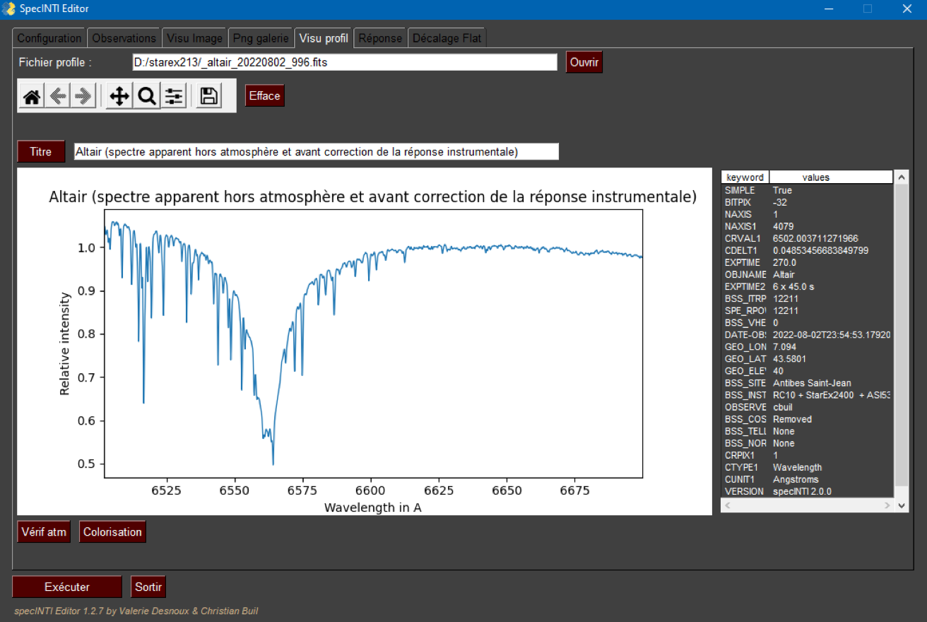
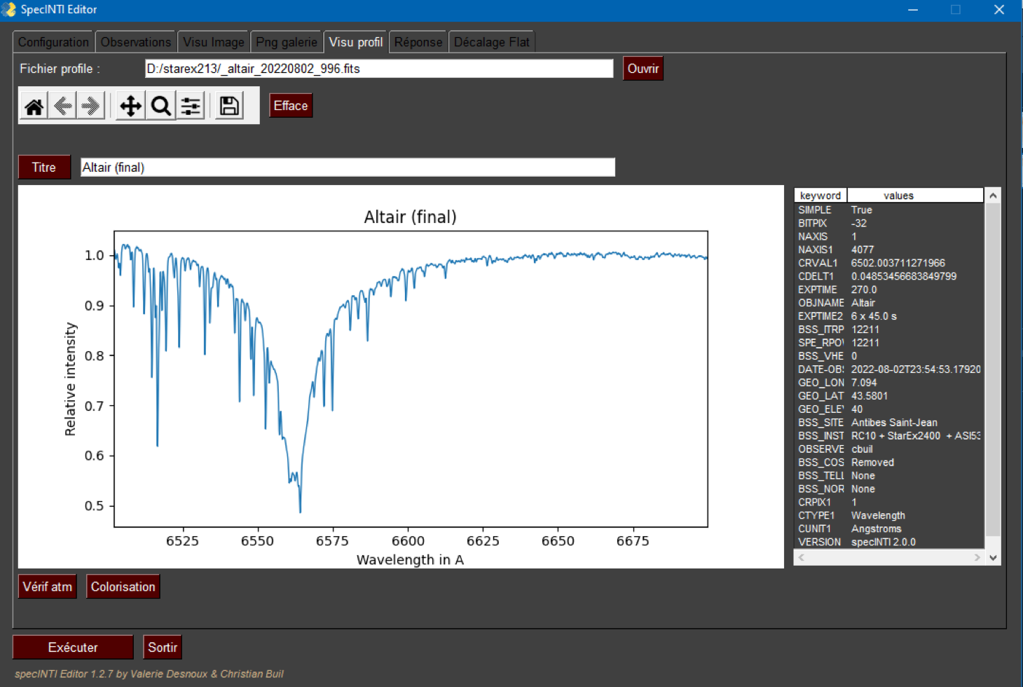
We now have an almost completely processed spectrum, saved in the working directory under the name "_altair_20220802_996.fits":
We say "almost" because, if we summarize the situation, this is the spectrum that you would see outside the atmosphere, but still affected by the distortions caused by the instrumental response, which has no chance of being a uniformly flat curve (the efficiency of the grating depends for example on the wavelength). The apparent spectrum in question is therefore the result of the operation :
apparent spectrum = (true spectrum) x (instrumental response)
The apparent spectrum (outside the atmosphere) is the one we have just calculated. We also have the true spectrum, it is the UVES spectrum. Therefore the calculation of the response is very simple, we reverse the previous equation:
To realize this division, we will use a function of specINT, which is called "_pro_div". The name is explicit: it is to divide two spectral profiles, a kind of arithmetic of spectra. If the operation to be performed is P3 = P1/P2, the syntax is as follows:
_pro_div: [P1, P2, P3]
With the elements of our example, this is what it gives (remember, the true star spectrum is the file « UVES_altair.FITS »):
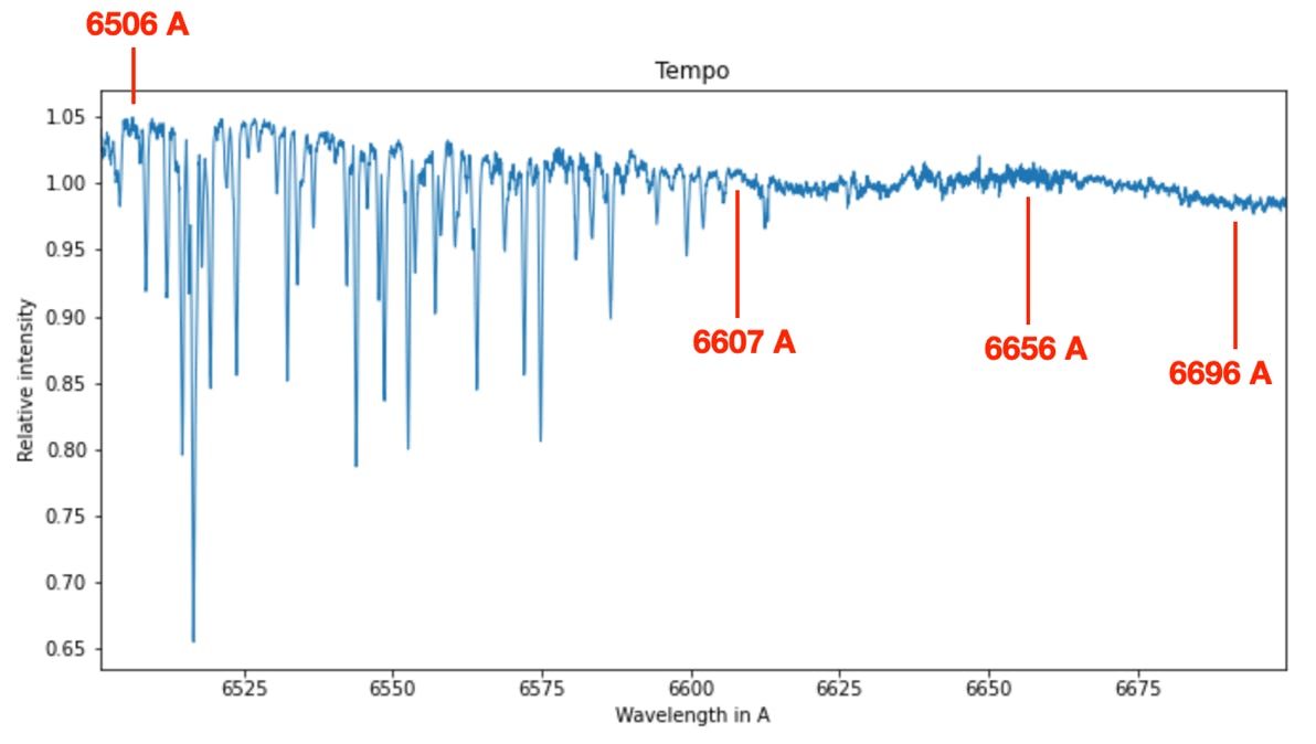
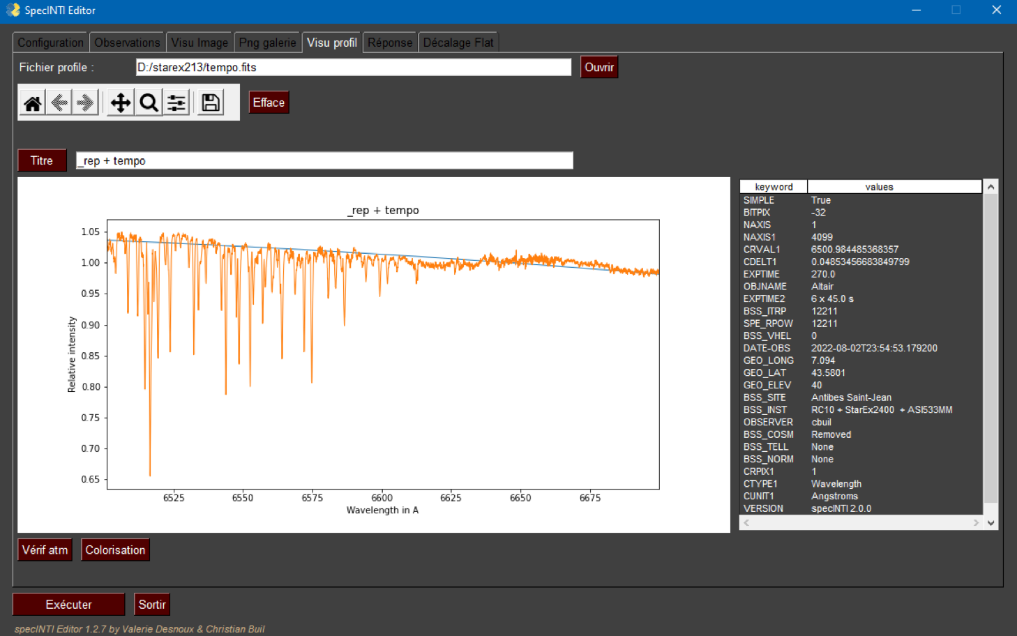
We decide to call the result of the division "tempo" and not "answer", you will quickly understand why. Here is the look of the "tempo" spectral profile:
The H-alpha hydrogen line has disappeared in what we could call an "instrumental response" (indeed the H-alpha line is present in the numerator as well as the denominator). Unfortunately the telluric lines (the spectrum of the H2O molecule) are well present in the dividend, because if they exist in our apparent spectrum, they are absent in the UVES spectrum.
However, if we disregard the H2O lines, we can see a slight downward slope from the blue side to the red side of the profile. This tendency is real and represents the instrumental response sought. At this stage we can synthesize a theoretical spectrum of water vapor and remove this in the "tempo" spectrum. This is feasible, and will be explained in the next section, but it is otherwise complex.
Another solution, much more expeditious, which I recommend here because the final result is satisfactory, is to generate a new profile by interpellating within the current profile from a very small number of points, avoiding telluric lines. We will use a new function, "_pro_fit", which simply adjusts a parabolic profile through only 4 points of the spectrum to interpellate, defined by their wavelengths.
The choice of points is flexible: you only need to avoid telluric lines and distribute them approximately evenly. Use the mouse pointer from the tab "Visu profile". For example:
Delete the previous function ("_pro_div") by replacing it with "_pro_fit", whose syntax is :
_pro_fit: [input, w1, w2, w3, w4, output]
For our example, this gives:
_pro_fit: [tempo, 6506, 6607, 6656, 6696, _rep]
Launch specINTI Editor with this line placed somewhere in the configuration file. The profile "_rep" is written in the working folder. This is our actual instrumental response. You can view it from the "Profile view" tab:
In this representation, we have in blue the profile of the true response (file " _rep ") and in orange, the profile of response of departure with the telluric lines. As it should be, the "response" profile is a monotonous curve, without asperities, which follows the general trend of the temporary "tempo" profile.
All that remains is to define a parameter in the configuration file that tells specINTI to use our instrumental response "_rep" (you can choose another name of course) to evaluate the final spectrum of the Altair star. This important parameter is called "instrumental_response". Delete the function "_pro_fit" and add in the final configuration file:
# ———————————————————————————
# Instrumental response file
# ———————————————————————————
instrumental_response: _rep
The final corresponding configuration file is : "conf_starex2400_mode0_demo3.yaml ».
Re-run specINTI, and you get the final profile of Altair, ready for publication - a spectrum out of the atmosphere and free of instrumental distortions:
Maybe you found this evaluation of the instrumental response tedious. You are a bit right, then software such as VisualSpec or ISIS perform the same arithmetic operations on the spectra in a more interactive way. We will say that the advantage of functions in specINTI is that you understand what you are doing and that the concept is extensible.
But above all, remember that the "_rep" file is now a constant. You use this same answer wherever you point in the sky. All this work has to be done only once, so the effort is worthwhile if you are an assiduous observer and if, of course, you don't disturb your spectrograph significantly. Thus, the configuration file "conf_starex2400_mode0_demo4.yaml", which contains the couple of parameters "corr_atmo" (calculation of the spectrum out of the atmosphere) and "instrumental_response" (removal of the instrumental response), can be used to successfully process all the spectra of our session (via the observation file "obs_nuit.yaml", see section 4.1) :
It gets even better: our "_rep" answer can be used from one night to the next, without being recalculated and without the need, during these nights, to observe reference stars as long as the "corr_atmo" parameter is present in your configuration file. This saves a lot of time and makes observations much easier. This is where specINTI and the way it is used shows all its power: you process blindly in a reliable way, sometimes even simultaneously with the observation if you wish. Using specINTI will become very easy once everything is set up.
Tip: Here is a particularly important and useful tip. You have just processed the starex213 session. Now you want to reduce the set of spectra of the starex214 session, with the data in question located in a working directory of the same name. Copy the _offset, _dark, _flat and _rep files from the starex213 folder to the starex214 folder, define the observation file of this last session, click on the "Run" button and everything is finished, you can move to the next session, and so on.
7.8.4 : Molecular atmospheric transmission
Correcting the apparent spectrum of sky objects to remove the molecular spectral signature left by the earth's atmosphere is a delicate operation. In the visible part of the spectrum, the lines responsible come from the molecules O2 (oxygen) and H2O (water vapor). The difficulty comes from the fact that these lines are numerous, sometimes organized in bands (called molecular bands), and that to this complexity of spectral content is added a variability. For example, the depth of the telluric lines depends on the humidity level of the atmosphere, which can of course vary according to the place (desert, tropical, mountain...), the season and even from hour to hour, as the night progresses. The height of the star pointed above the horizon modifies the air mass crossed and therefore also the contrast of the telluric lines.
What is the interest to tackle the suppression of telluric lines? First, these lines disturb to varying degrees the search for the instrumental response, as we have seen previously. These indentations in the spectrum, absent if we observe the stars outside the atmosphere, can be sources of accidental distortions in the spectral profile. But the most annoying thing is that they sometimes modify the spectrum of stars to the point of making it difficult to analyze.
Here is a typical example of this last point. The following graph shows three high resolution spectra of the star Spica (alpha Vir) around the Halpha line, taken at three different dates:
Spica is in fact a spectroscopic double with a rather strong amplitude in radial velocity and short period. Due to the variable radial velocity of the stars of the pair around a common center of gravity, the stellar lines are shifted periodically towards the red and then towards the blue. These three spectra clearly show the displacement of the Halpha line with respect to the fixed telluric lines, as well as the narrow lines coming from the molecules of the atmospheric water vapor. The concern comes from the fact that the Halpha line, with little contrast in this star, is bordered by telluric lines that hinder an accurate measurement of the Doppler effect.
The telluric lines can be numerically removed, as shown by the curves of the same spectra after the operation:
The spectra are such as one would observe them in the absence of the terrestrial atmosphere. The Halpha line is revealed as it really is, without the atmospheric interference.
It is important to note that removing the telluric lines can have a significant impact on the observed spectra, and it is therefore often requested to keep them in the data provided, except in the context of specific treatments. The most critical areas of the spectrum impacted by telluric lines are in the yellow and red, especially around the doublet of sodium and the Halpha line of hydrogen.
Complex software tools exist to model the atmosphere and its transmission, such as HITRAN, but it is difficult to obtain a faithful spectrum of the atmosphere based only on a parametric analysis.
The specINTI software offers the possibility to remove the telluric H2O lines in the visible part of the spectrum in an automatic way, thus simple. This approach is based on the use of precalculated synthetic molecular spectra, available in a spectra bank downloadable from the ESO Sky Model Calculator website: https://www.eso.org/observing/etc/bin/gen/form?INS.MODE=swspectr+INS.NAME=SKYCALC
We have extracted a number of molecular spectra of the atmosphere, formatted for processing with specINTI. This spectra bank is available in a ZIP archive, which you can download from this link: atmo_molecular.zip
It is recommended to create a folder « atmo_molecular » in the specINTI installation directory to store the molecular spectra extracted from the ZIP archive. These spectra are in FITS format and cover a spectral range from 3000 to 11000 A, with a step of 0.1 angstrom for the spectrum "_molecular_30mm.fits", for example. The special series of spectra whose name ends with "HR" covers a smaller spectral range, but with a finer step size of 0.02 A, suitable for processing spectra with high spectral resolution (R>10000).
Here is for example the aspect of an extract of the spectrum « _molecular_30mm.fits » :
The many fine lines are produced by the H2O and O2 molecules of our Earth's atmosphere, the famous telluric lines. Attention, this is a spectrum called "infinite resolution" (or almost). It is not precisely the aspect observed with our spectrographs, which have a limited resolution power.
The most expeditious way, and surely your favorite, to erase telluric lines from a star spectrum takes the form of a very simple function, called "pro_telluric". It has the following parameters:
"spectro_molecular" refers to one of the ESO spectra contained in the "atmo_molecular" directory. For most situations, don't ask too many questions and choose the median spectrum "_molecular_80mm_HR". "Input spectrum" is the name of the spectrum to be processed, and "output_spectrum" is the spectrum of the object after removing telluric lines.
Here is how to use this function - it takes two lines in a configuration file that you name as you like.
For example, if we want to remove the telluric lines from a processed spectrum correctly calibrated in wavelength named « _alphadra_20230505_807 », we simply write in a dedicated configuration file :
Below, on the left, the spectrum of the Halpha line in the alpha star Dra before the removal of the telluric lines H2O, on the right after the removal.
The « _pro_telluric » function is very effective when you need to remove telluric lines from a spectrum for one reason or another.