specINTI & specINTI Editor
11 : In the privacy of the observation file
In the previous sections, we have seen how to write the observation file through the "Observations" tab of the specINTI Editor interface. This file, after saving, is found in the current working folder with a name ending with the extension .yaml. In fact, it conforms to the YAML "standard", known in the computer world for exchanging parameters between applications. You can perfectly create and edit this file with a simple word processor. It can also be written by a third party software, for example the acquisition software itself as we observe during the night. Here are some explanations on the internal constitution of this observation file in case you want to start programming. The indicated layout is a kind of standard for specINTI, which must be respected to be understood by the latter.
Here is a typical content:
# *******************************************************
Altair:
# *******************************************************
- Altair # catalog name
- altair- # generic target file name
- 13 # number of target spectral images
- altair_neon- # generic spectral lamp files name
- 1 # number of spectral lamp images
- altair_tung- # generic flat lamp files name
- 18 # number of flat images
- n900- # generic dark files name
- 16 # number of dark images
- o- # generic offset files name
- 25 # number of offset files name
- none # optical atmospheric transmission
# *******************************************************
First of all, note that you can insert comments wherever you want, which improves readability. A comment starts with the character " # " .
Each target object to be processed has a block of data associated with it. So there are as many blocks as there are observed objects. The beginning of a block is marked by a text (or key) followed by a colon ":".
The text in the preamble is only used to delimit the current block from the previous or following blocks. Lower case or upper case, or even spaces are possible. For example, you could have written "My beautiful observation of Altair:".
My beautiful observation of Altair:
Then come 12 lines (this number is imposed, excluding comments) describing the actual observation of a given target, in this case the spectrum of the star Altair (this is an example). Each line must begin with a dash " - " followed by at least one blank. The order of these lines must imperatively be respected in relation to their meanings.
Line 1: the "official" designation of the star, found in the catalogs, and not included in the CDS. For this star we could still choose "HD 187642" or "53 Aql", and we would then write,
- HD187642
or
- 53 Aql
Lines 2 and 3: the generic name of the raw images in FITS format of the star to be processed and the corresponding number of images in the sequence. In the example, the image files of the sequence are named on the storage disk: altair-1, altair-2..., altair-13. For the sake of readability, it is recommended that the generic name given to the image files end with a dash, as in this example.
Lines 4 and 5: the generic name of the spectral calibration files and their number. Note that you are absolutely free to choose the name given to the file. In the example, there is only one calibration file, called "altair_neon-1".
Lines 6 and 7: the generic name of the flat-field images and their number. Here we have the sequence altair_tung-1, altair_tung-2..., altair_tung-18. We will explain later how these images were acquired. These images are combined by specINTI to produce a "master flat", saved under the reserved name "_flat" in the working folder.
Lines 8 and 9: the generic name of the dark signal images and their number. In the example, one uses 16 images of dark exposed 900 seconds in the darkness, which one decided to call: n900-1, n900-2..., n900-18. These images will be combined automatically by specINTI in order to build a " dark master " (and the file " _offset ").
Lines 10 and 11: the generic name of the images of the offset signal and their number. Here: o-1, o-2..., o-25. These images are taken in the dark with a very short exposure time. specINTI uses these individual images to automatically produce a "master offset" image (and the "_dark" file).
Line 12: the name of a FITS file containing the atmospheric transmission spectrum at the time of the observation and in the line of sight of the target. For simplicity, we do not use such a file here, and for this reason we indicate the name "none".
If these 12 lines are imperative, it is possible that you do not have all the necessary files. For example, you forgot to acquire the flat-field images (which is not good!). How can you do this?
The trick is to specify a zero number of images for the corresponding sequence. For example, let's assume that you don't have any flat-field images for this observation. In this case you would write something like :
- altair_neon- # generic spectral lamp files name
- 1 # number of spectral lamp images
- altair_tung- # generic flat lamp files name
- 0 # number of flat images
- n900- # generic dark files name
- 16 # number of dark images
The generic name of the sequence does not matter, and you could write :
- pas de flat-field # generic flat lamp files name
- 0 # number of flat images
specINTI will always process your spectra with the data it has, but be careful, the availability of the "flat, dark, offset" file trio is really the rule to exploit your observations well.
The observation file reveals its power when you understand that it is possible to process several targets in a row in a fully automatic way. All you have to do is copy and paste the target blocks, the file structure being repetitive. For example:
# *******************************************************
Altair:
# *******************************************************
- Altair # catalog name
- altair- # generic target file name
- 13 # number of target spectral images
- altair_neon- # generic spectral lamp files name
- 1 # number of spectral lamp images
- altair_tung- # generic flat lamp files name
- 18 # number of flat images
- n900- # generic dark files name
- 16 # number of dark images
- o- # generic offset files name
- 25 # number of offset files name
- none # optical atmospheric transmission
# *******************************************************
# *******************************************************
Vega:
# *******************************************************
- Vega # catalog name
- vega- # generic target file name
- 18 # number of target spectral images
- vega_neon- # generic spectral lamp files name
- 1 # number of spectral lamp images
- altair_tung- # generic flat lamp files name
- 18 # number of flat images
- n900- # generic dark files name
- 16 # number of dark images
- o- # generic offset files name
- 25 # number of offset files name
- none # optical atmospheric transmission
# *******************************************************
Here specINTI will first compute the spectrum of the star Altair, then continue with the processing of the spectrum of the star Vega. You can include as many target blocks as you wish in the observation file.
Note in the example that for the processing of the star Vega, we use the same calibration data (same flat-field, same dark, etc). This is not mandatory, but it is often the case in practice.
As things are written, for each object, specINTI calculates the master images of flat-field, dark and offset, each block being independent of the others. This calculation is fortunately fast, but there is a more elegant way to write the observation "batch" file, as the following example shows:
# *******************************************************
Altair:
# *******************************************************
- Altair # catalog name
- altair- # generic target file name
- 13 # number of target spectral images
- altair_neon- # generic spectral lamp files name
- 1 # number of spectral lamp images
- altair_tung- # generic flat lamp files name
- 18 # number of flat images
- n900- # generic dark files name
- 16 # number of dark images
- o- # generic offset files name
- 25 # number of offset files name
- none # optical atmospheric transmission
# *******************************************************
# *******************************************************
Vega:
# *******************************************************
- Vega # catalog name
- vega- # generic target file name
- 18 # number of target spectral images
- vega_neon- # generic spectral lamp files name
- 1 # number of spectral lamp images
- _flat # generic flat lamp files name
- 0 # number of flat images
- _dark # generic dark files name
- 0 # number of dark images
- _offset # generic offset files name
- 0 # number of offset files name
- none # optical atmospheric transmission
# *******************************************************
The way to understand it is that when processing the first target (Altair), specINTI generates the master files flat-field, dark and offset, and saves them in the working directory using the respective reserved names "_flat", "_dark" and "_offset". If you examine your data storage system, you will find these files.
For the processing of the second object, "Vega", we make sure to tell specINTI to use the pre-calculated master images and not to re-calculate the entire master images. To do this, you just need to specify the name reserved for the corresponding lines and set the value 0 for the number of images. In this situation, the calculation is of course faster.
This process is flexible, because the files in question may well have been created in a previous session, a day ago, a month ago... You just need to copy these master images to the current working folder.
Tip: suppose that in a long sequence of stars described in the observation file, you do not want to process the data of one or more of these objects. There is no need to write a specific observation file, in which you would have to delete the blocks of unwanted objects. The easiest way to do this is to specify a zero number for the sequence of "science" images that you do not want to process. Thus, in the example :
# *******************************************************
Altair:
# *******************************************************
- Altair # catalog name
- altair- # generic target file name
- 0 # number of target spectral images
- altair_neon- # generic spectral lamp files name
- 1 # number of spectral lamp images
- altair_tung- # generic flat lamp files name
- 18 # number of flat images
- n900- # generic dark files name
- 16 # number of dark images
- o- # generic offset files name
- 25 # number of offset files name
- none # optical atmospheric transmission
# *******************************************************
# *******************************************************
Vega:
# *******************************************************
- Vega # catalog name
- vega- # generic target file name
- 18 # number of target spectral images
- vega_neon- # generic spectral lamp files name
- 1 # number of spectral lamp images
- altair_tung- # generic flat lamp files name
- 18 # number of flat images
- n900- # generic dark files name
- 16 # number of dark images
- o- # generic offset files name
- 25 # number of offset files name
- none # optical atmospheric transmission
# *******************************************************
specINTI skips the processing of the Altair star, and goes directly to the processing of the Vega star. This trick is useful for fine-tuning the observation file or for resuming the processing in case of a failure on only a few objects, thus isolated in the observation file. This principle of zero image number can also be applied from the specINTI Editor interface.
12 : Calibration modes’
Some of the calibration modes that can be used with specINTI to calibrate wavelength spectra have been described in the previous sections. These modes cover most of the needs according to situations closely related to the way of operating the spectrograph or the type of object observed. The mode is indicated to the software through the "calib_mode" parameter. Here is the complete list, with a brief description.
Mode #0 : This is the mode that can be considered as "standard" in spectrography. You use a calibration lamp with emission lines (neon, argon, mercury...) and if possible, you take a spectrum of this lamp before and after the observation session of the science images of the target object. specINTI uses the spectrum(s) of this lamp to automatically calculate the calibration polynomial (dispersion law that relates the image pixel numbers to wavelengths) and applies it to the "science" data. Hereafter the characteristic spectrum of a spectral calibration lamp with emission lines (extracted from the spectrum of a discharge lamp containing neon gas):
Mode #1 : You have already evaluated the terms of the characteristic spectral calibration polynomial of your spectrograph - a kind of hardware constant. For this evaluation you have used the spectrum of a spectral lamp with emission lines or absorption lines of a hot star of spectral type A or B. This dispersion law can be calculated with a software other than specINTI (VisualSpec, ISIS, ...) or with specINTI itself (see section 5.4). This polynomial is directly applied to the data to be processed and you do not need to use a calibration source during the whole observation session. This mode #1 is called "experimental" or "test" mode, because it is difficult to use normally since nothing says that the calibration function is stable during the session, depending on the temperature, the pointing of the telescope... Using only the generic dispersion polynomial can lead to significant calibration errors. However, there are situations where the #1 mode can be very useful. For example, in planetary spectrography, when one seeks to compare the spectrum of several regions of the surface, being able to fix the calibration polynomial facilitates considerably the analysis.
Mode #2 : This mode is mixed between modes #0 and #1 previously described. The idea is that a phenomenon of mechanical bending of the spectrograph, variable according to the point of the sky pointed, or following a thermoplastic deformation, leads to the first order translation of the image of the spectrum on the detector. Let us assume the following calibration polynomial of order 3:
Lambda = A3 x X^3 + A2 x X^2 + A1 x X + A0
with lambda, the wavelength, X the rank of a pixel in the image along the spectral axis and (A0, A1, A2, A3), the coefficients of the calibration polynomial.
It is assumed (which is also verified) that at first order, if the instrument undergoes a mechanical or thermal deformation, it is the term A0 that is mostly affected. This means that despite these accidents, the spectrum remains consistent with itself during the session (or several sessions) except for a translation. For example, its average scale (A1 term) does not change. We say that the spectrum remains affine. The higher order terms are also reasonably constant as long as the translation is not considerable (say a few pixels to a few tens of pixels, as a general rule).
Ultimately, calibration mode #2 consists of: (1) to evaluate all the terms of the calibration polynomial only once, by observing a broad band spectral lamp or possibly, for lack of a better term, the lines of the Balmer series of the A or B type stars, whose positions are well defined and known, (2) to consider that this polynomial is an instrumental constant if the spectrograph is not deregulated, (3) to use a calibration source (emission line lamp) for each observed star in order to recalibrate only the A0 term (only one line is needed, but you can use several, and in this case, specINTI computes an average value of the A0 term, which is more accurate).
Mode #2 solves a difficult and quite common problem: it is the solution when your spectral lamp on the telescope does not offer enough lines to cover the whole spectral range observed by the spectrograph, or when the lines of the lamp are not very intense and badly distributed. This mode #2 is particularly useful if you work in low spectral resolution with a spectrograph covering a wide range of wavelengths.
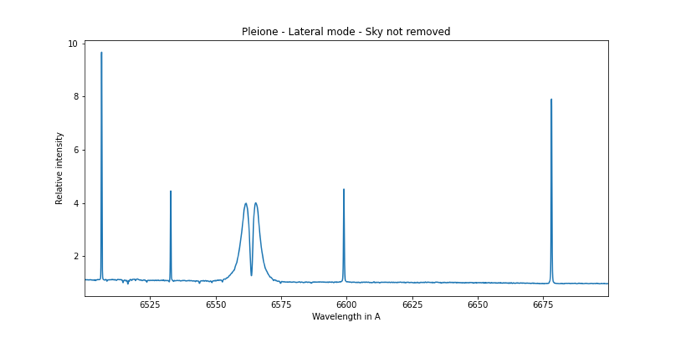
Mode #3 : specINTI performs a spectral calibration with the lines of a standard lamp that illuminates the spectrograph while observing the stars. The calibration illumination ideally takes the form of a permanent low intensity illumination of the telescope mirror while observing the "science" targets (the brightness of this calibration source is adjusted so that after a long exposure time its electronic signal represents only a fraction of the sensor dynamic range). Each elementary exposure on the targets is therefore associated with a calibration spectrum, which is printed in the spectrum of the target itself. There is indeed a superposition of two spectra in the end. This is called a lateral calibration mode because the calibration emission lines appear on either side of the spectrum trace. During the treatment process, this calibration spectrum is erased from the science spectrum. Beforehand, the calibration spectrum is analyzed to automatically extract the calibration polynomial perfectly adapted to the data to be processed.
The interest of mode #3 is the simultaneous taking of the target spectrum and the spectral calibration source. Thus, mechanical bending or thermal deformation no longer have an effect on the quality of the spectral calibration. This opens the way to light and economical spectrographs, such as the Star'Ex instrument. The lateral mode as described is a real breakthrough in the world of amateur spectrography, which can be approached in a completely different way. This way of doing is not new: with different technical means, but for an identical goal, it is thanks to the calibration parallel to the science shots that one realizes radial velocity measurements of very high precision, for example at the origin of the discovery of exoplanets. The #3 mode is more particularly adapted to spectrography at high spectral resolution (R>10000).
The image below shows an image of the spectrum of the star Pleione (in Messier 45) obtained with a 100 mm diameter telescope is a Star'Ex spectrograph operated with high spectral resolution. We are well in lateral mode, because in superposition to the spectrum of the star (the horizontal line), in the same image, we have a comb of line coming from a neon lamp (the vertical lines):

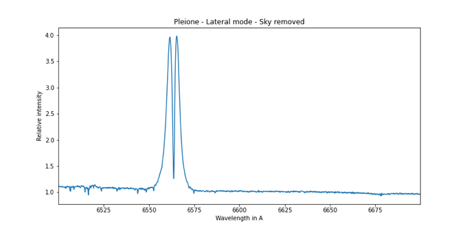
This same Pleione spectrum, but in the form of a spectral profile, while the calibration lines have not been removed:
Below is the spectrum after the software removal of the calibration lines. Its appearance has now become usual (parameter "sky_remove" taking the value 1 in the configuration file, which is also the default behavior of specINTI).
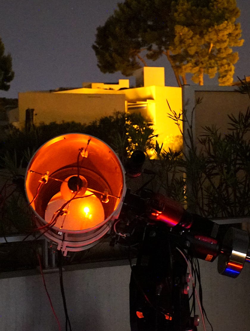
In the image opposite, the illumination of the mirror of a Newton telescope of 250 mm in diameter by 4 neon lamps fixed on the branches of the secondary spider.
Mode #4 : This mode is intermediate between mode #0 and mode #3. The terms of the calibration polynomial are evaluated by choosing a spectral lamp rich in lines (possibly on a table, outside the telescope, thus with relatively heavy means, see section 3). These coefficients are then considered as constants of the instrument, or at least, values that are not updated frequently. specINTI then uses the lateral spectrum for the recalibration of the term A0 of the polynomial, which can evolve as a function of time or of the telescope pointing.
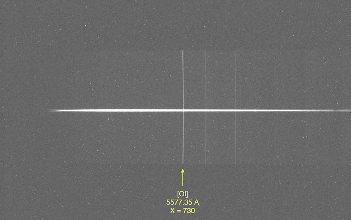
Mode #4 can be used when observing under a polluted sky, in a city, in the presence of sodium or mercury urban lighting lamps: this pollution source is then used as an advantage since it provides the equivalent of a free and permanent standard lamp. This is one of the rare cases where light pollution is used for something positive in astronomy! If the observatory is very isolated from light pollution, it is sometimes possible to exploit lines emitted by the upper atmosphere, in particular the green line at 5577 A, always present when working in low resolution. This use of artificial or natural lines, coming from the sky itself, is of course very simple, but also accurate, without any calibration bias, since the rays coming from the science target and the calibration source follow the same optical path, which is the Holy Grail in terms of calibration.
To illustrate, the image below is that of the 2D spectrum of a star made in a desert area in Chile (2SPOT) with an Alpy600 spectrograph: we use here the atmospheric fluorescence line at 5577 A, always more or less visible (which gives the green color to the aurora borealis, by the way), to tare the spectra (adjustment of the A0 term) :
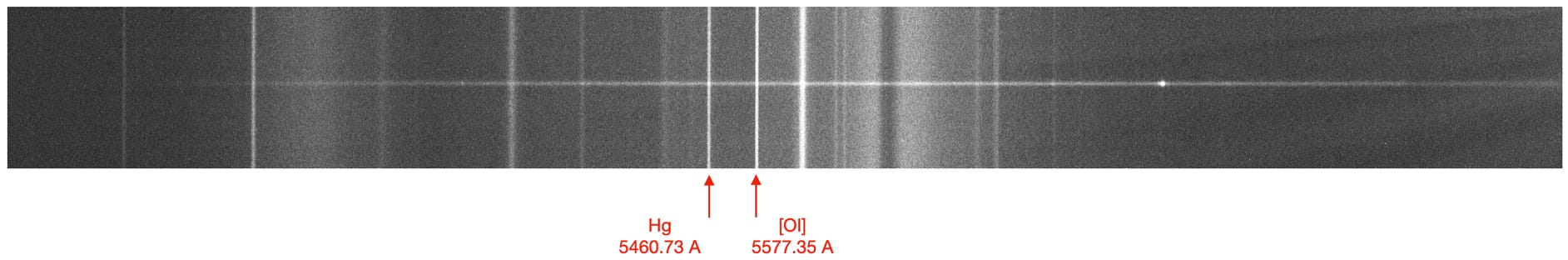
Another example on a low resolution Star'Ex spectrum of the star HL Tau (note the emission of the H-alpha line in the right part), this time realized in urban environment. The lines that can be used for calibration in mode 4 can be those of sodium or better, mercury (Hg) produced by urban lighting.
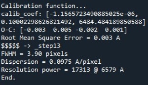
Here is a typical example of a configuration file using mode 4, with in red, the differences with respect to mode 3 described in section 4 (mainly the wavelengths and position of the lines used to calculate the parameter A0 of the dispersion polynomial, currently worth 3773.712 A ("calib_coef" parameter), but which will be modified by the software following the observation of these lines :
# *****************************************************************
# Sol'EX 300 t/mm configuration - Newton 250 f/4 - 19 micron slit
# Calibration mode 4
# *****************************************************************
# ---------------------------------------------------
# Working directory
# ---------------------------------------------------
working_path: /Volumes/Samsung_T5/starex_16102021
# ---------------------------------------------------
# Processing batch file
# ---------------------------------------------------
batch_name: obs_hltau
# ---------------------------------------------------
# Spectral calibration mode
# ---------------------------------------------------
calib_mode: 4
# ----------------------------------------------------------------
# Coefficients of the spectral calibration polynomial
# ----------------------------------------------------------------
calib_coef: [-1.336316e-9, 7.98424e-6, 0.96625, 3773.712]
# ---------------------------------------------------
# binning width
# ---------------------------------------------------
bin_size: 40
# ---------------------------------------------------
# Sky background calculation areas
# ---------------------------------------------------
sky: [150, 24, 24, 150]
# ---------------------------------------------------
# x-boundaries for geometric measurements
# ---------------------------------------------------
xlimit: [1500, 2500]
# ----------------------------------------------------------------
# Width in pixels of the line search area
# ----------------------------------------------------------------
search_wide: 40
# ---------------------------------------------------
# Lengths in calibration A-waves (required)
# ---------------------------------------------------
wavelength: [5577.35, 5460.73]
# ---------------------------------------------------
# Line positions in pixels (required)
# ---------------------------------------------------
line_pos: [1857, 1738]
# ----------------------------------------------------------------
# Name of the instrumental response file
# ----------------------------------------------------------------
instrumental_response: response
# ----------------------------------------------------------------
# Median filter core size
# ----------------------------------------------------------------
kernel_size: -3
# ----------------------------------------------------------------
# Gaussian filtering
# ----------------------------------------------------------------
sigma_gauss: 1.0
# ----------------------------------------------------------------
# Sky background evaluation mode
# ----------------------------------------------------------------
sky_mode: 1
# ----------------------------------------------------------------
# Profile extraction mode
# ----------------------------------------------------------------
extract_mode: 1
# ----------------------------------------------------------------
# Read noise in e-
# ----------------------------------------------------------------
noise: 1.5
# ----------------------------------------------------------------
# Electronic gain in e-/ADU
# ----------------------------------------------------------------
gain: 0.0418
# ----------------------------------------------------------------
# Unit normalization area
# ----------------------------------------------------------------
norm_wave: [6640, 6660]
# ----------------------------------------------------------------
# Profile cropping area
# ----------------------------------------------------------------
crop_wave: [3850, 7000]
# ----------------------------------------------------------------
# Longitude of the observation place
# ----------------------------------------------------------------
Longitude: 7.0940
# ----------------------------------------------------------------
# Latitude of the observation site
# ----------------------------------------------------------------
Latitude: 43.5801
# ----------------------------------------------------------------
# Altitude of the observation point in meters
# ----------------------------------------------------------------
Altitude: 40
# ----------------------------------------------------------------
# Observation site
# ----------------------------------------------------------------
Location: Antibes St-Jean
# ----------------------------------------------------------------
# Description of the instrument
# ----------------------------------------------------------------
Inst: Newton250 + SolEx (300) + ASI183MM
# ----------------------------------------------------------------
# Observer (optional)
# ----------------------------------------------------------------
Observer: cbuil
13 : Special modes
13.1 : Mode -1 : Evaluation of the dispersion polynomial with an absorption spectrum
Note first that the special modes are distinguished by a negative numbering.
The -1 mode allows to calculate the spectral dispersion polynomial of the degree of choice from the observed position of the Balmer lines (hydrogen absorption spectrum) from specINTI. The ideal for this is to observe a hot star of spectral type A or B, because these lines are intense. Here is the procedure. Write a configuration file as follows (extract):
# ---------------------------------------------------
# Spectral calibration mode
# ---------------------------------------------------
calib_mode: -1
# ---------------------------------------------------
# Wavelength of Balmer lines
# ---------------------------------------------------
fit_wavelength: [3889.05, 3970.08, 4101.75, 4340.48, 4861.34, 6562.81]
# ---------------------------------------------------
# approximate position of the Balmer lines in pixels
# ---------------------------------------------------
fit__posx: [259, 283, 318, 386, 528, 1012]
# ---------------------------------------------------
# Search line wide zone
# ---------------------------------------------------
seach_wide: 8
# ---------------------------------------------------
# Degree of the calibration polynomial
# ---------------------------------------------------
fit_order: 3
The parameters fit_wavelength and fit_posx represent respectively the wavelengths of the chosen Balmer lines and their approximate pixel coordinates in the image. We choose the degree of the polynomial through the poly_order parameter (here the degree 3). Remember that if n is the number of Balmer lines chosen, the degree cannot exceed n-1. The processing is done on a star in which the Balmer lines are well contrasted, for example :
# *********************************************************
HD 223352:
# *********************************************************
- HD 223352 # catalog name
- HD 223352- # generic target file name
- 11 # number of target spectral images
- HD 223352_Neon- # generic spectral lamp files name
- 1 # number of spectral lamp images
- flat- # generic flat lamp files name
- 32 # number of flat images
- Dark_1200- # generic dark files name
- 5 # number of dark images
- Dark_bias- # generic offset files name
- 17 # number of offset files name
- none # optical atmospheric transmission
The processing stops with the display of the calculated dispersion polynomial (the processing of the star is not complete):
Computed calibration coefficients:
-2.6658628005617566e-07, 0.0003809274285578211, 3.4241240905489154, 2991.942942846281
Residue = 0.04 A
End.
You can now report these items in the configuration file for the actual processing:
# ----------------------------------------------------------------
# Spectral calibration coefficients
# ----------------------------------------------------------------
calib_coef: [-2.6658628005617566e-07, 0.0003809274285578211, 3.4241240905489154, 2991.9429428]
13.2 : Mode -2 : Evaluation of the dispersion polynomial with an emission spectrum
Like the -1 mode, the -2 mode allows to calculate the spectral dispersion polynomial of the degree of one's choice, but now by exploiting an emission spectrum, coming for example from a reference spectral lamp.
The structure of the observation file will be for example :
# *********************************************************
POLYNOME DE DISPERSION A PARTIR D’UNE LAMPE NEON:
# *********************************************************
- Lampe neon # catalog name
- neon- # generic target file name
- 4 # number of target spectral images
- none # generic spectral lamp files name
- 0 # number of spectral lamp images
- none # generic flat lamp files name
- 0 # number of flat images
- n600- # generic dark files name
- 16 # number of dark images
- o- # generic offset files name
- 29 # number of offset files name
- none # optical atmospheric transmission
Here, neon-1, ... neon-4 are the spectrum images of a neon lamp.
The characteristic configuration file is then written as follows (extract):
# ---------------------------------------------------
# Spectral calibration mode
# ---------------------------------------------------
calib_mode: -2
# ---------------------------------------------------
# Wavelength of Balmer lines
# ---------------------------------------------------
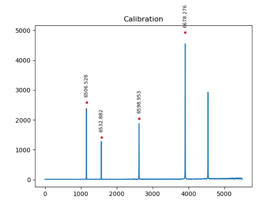
wavelength: [6506.53, 6532.88, 6598.95, 6678.28, 4861.34]
# ---------------------------------------------------
# Approximate position of the Balmer lines in pixels
# ---------------------------------------------------
line_pos: [1163, 1574, 2625, 386, 528, 3911]
# ---------------------------------------------------
# Degree of the calibration polynomial to evaluate
# ---------------------------------------------------
poly_order: 2
# ---------------------------------------------------------------
# Typical vertical position of the spectrum trace
# ---------------------------------------------------------------
posy: 345
# ---------------------------------------------------------------
# Line binning height, between 10 and 100 pixels
# ---------------------------------------------------------------
bin_size: 40
# ---------------------------------------------------------------
# Line search width relative to the specified position (optional)
# ---------------------------------------------------------------
search_wide: 40
# ---------------------------------------------------------------
# Definition of the calculation areas to find the line plant angle
# ---------------------------------------------------------------
sky: 40
# ---------------------------------------------------------------
# Typical tilt angle found on the spectra trace (optional)
# ---------------------------------------------------------------
tilt: -0.021
# ---------------------------------------------------------------
# Radius of curvature of the smille (optional, but recommended)
# ---------------------------------------------------------------
smile_radius: -17000
# ---------------------------------------------------------------
# Gaussian filtering (optional)
# ---------------------------------------------------------------
sigma_gauss: 0.5
The parameters « wavelength » and « line_pos » are mandatory. They represent respectively the wavelengths of the selected emission lines and their approximate pixel coordinates in the image. Note that the « auto_calib » parameter is not operational in this -2 mode, but also note that specINTI Editor offers an interactive way to generate the list of line coordinates in the calibration image (the first one for example if it is a sequence) by a simple "Alt - click" with the mouse. Then you just have to copy and paste this list as an argument to the « line_pos » parameter. The « posy » parameter, mandatory, specifies the approximate vertical coordinate in pixels of the trace of the stellar spectra to be calibrated (in general, the center of the image along the vertical axis). It is also necessary to include the parameter « bin_size » which indicates on which height of the emission lines the calculation is made. The typical value is about 40 pixels to obtain a good signal to noise ratio. The definition of the « sky » parameter is necessary to evaluate the slant angle of the emission lines. You are also free to use the parameters « ilt », « smile_radius » or « sigma_gauss » to test the effect of Gaussian smoothing on the spectral resolution.
The processing stops with the display of the calculated dispersion polynomial and the evaluation of the spectral resolution power. More precisely, here is a typical output of the special -2 mode:
You can use the calib_coef: line as is... it is ready to use to calibrate your spectra. You can see the mathematical evaluation error of the polynomial (better than 1/100 angstrom), the characteristic FWHM of the lines, the value of the spectral dispersion as well as the resolving power on the basis of your standard lamp. All this information will surely be useful to you. A key application of the special -2 mode is to support the mode 4 lateral calibration of spectra.
13.3 : Mode -3 : Evaluation of the noise and gain of a camera
The -3 mode allows you to calculate the gain and the reading noise of your camera. These values are useful when the optimal extraction mode (Horne) is requested.
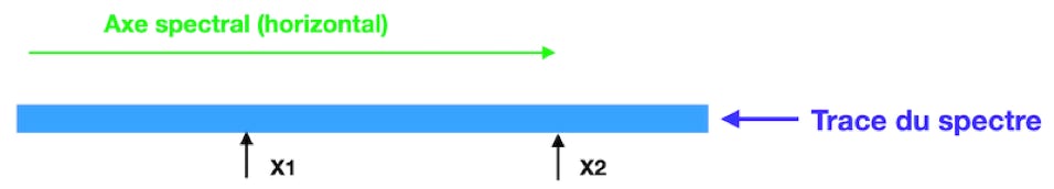
The calculation is made from two flat-field images and two offset images (at least), in a common area of the images associated with a relatively high and uniform signal level in the flat-field. This area is delimited by a rectangle of pixel values for which the coordinates of the opposite corners (X1, Y1) and (X2, Y2) are given. These values are provided to specINTI through the « area » parameter, in the form :
area: [x1, y1, x2, y2]
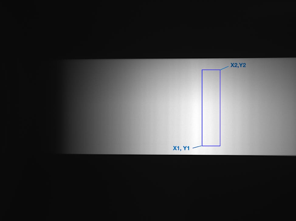
Definition of the surface of the flat-field image from which specINTI will calculate the gain and noise of the camera.
Here is how to fill in the configuration file:
# ---------------------------------------------------
# Spectral calibration mode
# ---------------------------------------------------
calib_mode: -3
# ---------------------------------------------------
# Wavelength of Balmer lines
# ---------------------------------------------------
area: [940, 350, 1000, 600]
Here is how to fill in the configuration file:
# *********************************************************
HD 223352:
# *********************************************************
- HD 223352 # catalog name
- HD 223352- # generic target file name
- 11 # number of target spectral images
- HD 223352_Neon- # generic spectral lamp files name
- 1 # number of spectral lamp images
- flat- # generic flat lamp files name
- 32 # number of flat images
- dark1200- # generic dark files name
- 5 # number of dark images
- offset- # generic offset files name
- 17 # number of offset files name
- none # optical atmospheric transmission
The software uses the flat-1, flat-2, offset-1, offset-2 images to calculate the gain and the reading noise. Here is an example of the output:
Camera gain = 0.250 e-/ADU - Read Out Noise = 3.73 e-
End.
13.4 : Mode -4 : Manual calculation of the spectral dispersion polynomial
Mode -4 fits a polynomial of the degree of choice, of the form lambda=f(x), with lambda a list of wavelengths, and x the pixel coordinate of these same lengths. The coefficients of the polynomial are returned in the output console.
The list of wavelengths is the content of the "fit_wavelength" parameter. The list of coordinates is the content of the "fit_posx" parameter. The degree of the polynomial is the argument of the "fit_order" parameter.
Example :
# ----------------------------------------------------------------
# Spectral calibration mode
# ----------------------------------------------------------------
calib_mode: -4
# ----------------------------------------------------------------
# Order of the dispersion polynomial to be evaluated
# ----------------------------------------------------------------
fit_order: 3
# ----------------------------------------------------------------
# Wavelengths of the standard lines
# ----------------------------------------------------------------
fit_wavelength: [3948.979, 4044.418, 4259.362, 5037.751, 5116.590, 5400.562, 5852.488, 6143.063, 6402.248, 6506.528, 6717.043, 7032.413, 7245.166, 7438.898, 7635.106]
# ----------------------------------------------------------------
# Coordinate of the standard lines in pixels in the image
# ----------------------------------------------------------------
fit_posx: [307, 369, 508, 1009, 1061, 1244, 1535, 1722, 1889, 1955, 2090, 2292, 2427, 2551, 2675]

13.5 : Mode -5 : extraction of the raw spectral profile
The -5 mode is very basic. It is used when you want to extract the raw profile of the object. By raw, we mean a profile not calibrated in wavelength, obtained by a simple binning in column. The intensities are those of the sum of all the spectra of the image list provided. The unit is the raw numerical count in the images. The sky background can be removed or not (the possibility of not removing it can be useful to extract the raw profile of a spectral lamp, for example).
A typical example:
# ---------------------------------------------------
# Working directory
# ---------------------------------------------------
working_path: D:/starex260
# ---------------------------------------------------
# Processing batch file
# ---------------------------------------------------
batch_name: regulus
# ---------------------------------------------------
# Spectral calibration mode
# ---------------------------------------------------
calib_mode: -5
# --------------------------------------------
# Binning width
# --------------------------------------------
bin_size: 30
# --------------------------------------------
# Sky background shrinkage
# --------------------------------------------
sky_remove: 1
# ---------------------------------------------------
# Sky background calculation areas
# ---------------------------------------------------
sky: [200, 22, 22, 200]
# ---------------------------------------------------
# Sky extraction mode
# ---------------------------------------------------
sky_mode: 0
# ---------------------------------------------------
# x-terminals for geometric measurements
# ---------------------------------------------------
xlimit: [400, 1700]
# ----------------------------------------------------------------
# Median filter pattern
# ----------------------------------------------------------------
kernel_size: -3
# ----------------------------------------------------------------
# Gaussian filtering
# ----------------------------------------------------------------
sigma_gauss: 1.0
# ----------------------------------------------------------------
# Goodies
# ----------------------------------------------------------------
check_mode: 0
Note the use of the optional parameter sky_remove, and the ability to filter images (kernel_size, sigma_gauss, and in this case, the profile is no longer quite raw - to get a profile as close as possible to the original content, remove these parameters from the configuration file).
14 : Parameters Reference Manual
This section is the reference manual for the configuration file. All possible parameters are described.
Although it is not mandatory, you can organize (and write) the configuration file by grouping the parameters into three separate sections:
- a section devoted to the parameters that you change when you move from one observation session to another (typically, the path of the working folder that contains the data to be processed).
- a section related to your preferences on how to process the spectra, preferences that are generally generic from one observation session to another (but that can also be specific to the processing of a particular object within the same session, but this case is rather rare).
- a section of parameters corresponding to the way you operate your acquisition software or your observatory (FITS file extension, your geographical coordinates). This information can be isolated, because it does not impact the quality of your processing.
This is the organization by section that we adopt in this reference manual to describe the parameters.
14.1 : Parameters related to the observation session
BATCH_NAME : Optional parameter. Specifies the name of the observation file (of type .yaml) present in the working folder to be processed. It is recommended that the batch_name parameter be defined in the configuration file. If this parameter is not present, specINTI assumes that the observation file has the file name: 'object.yaml'.
Example:
batch_name: obs_qrvul
WORKING_PATH : Mandatory parameter. Path to the folder containing the images to be processed and the observation file (.yaml). This folder is called "working directory".
Example under maxOS :
working_path: /Volumes/Samsung_T5/specINTI_test/300/
Example under Windows :
working_path: c:\observations\nuit_051221\
14.2 : Parameters related to the spectra
ATMO_BLUR : Optional parameter.. If this parameter is defined, the molecular atmospheric transmission file transmitted to specINTI (via the observation file) undergoes a Gaussian filtering (smoothing) with a FWHM equal to the value of this parameter. This possibility allows to adjust the spectral resolution of the atmospheric transmission model (a line file) to the resolution of the processed spectra.
Example :
atmo_blur: 25
AUTO_CALIB : Optional parameter. Performs an automatic search for calibration lines (only neon gas) and a spectral calibration, also automatic. This function can be used in the standard calibration modes (#0 or # 2) as well as in the lateral modes (#3 and #4). The search for lines is limited by the two wavelengths passed in a list. BUT BEWARE: auto_calib is only functional in high spectral resolution (2400 t/mm grating when using Star'Ex for example or a Lhires III), in a spectral range where the spectral lines are well distributed over the whole width of the recorded spectrum, and of course, when the calibration source is a neon type lamp.
Example :
auto_calib: [6450, 6750]
Example :
auto_calib: [6450, 6750]
AUTO_CALIB_TH : Optional parameter. Detection threshold of the calibration lines in ADU for the auto_calib function. The spectral lines used are those whose peak intensity exceeds this threshold. Normally, it is not necessary to add the auto_calib_th parameter, (the threshold is automatically calculated by the software), but in some rare circumstances it may be useful to define it manually.
BIN_FACTOR : Optional parameter. Binning factor (agglomeration) of the final spectrum points. For example, if the value of this parameter is 2, the points are added 2 by 2 (specINTI calculates an average value). The spectral binning allows to increase the signal to noise ratio, when it is low in the initial spectrum, but of course, the resolution power decreases (in a proportion determined by the value of the sampling relative to the spectral sharpness - there is not necessarily a direct relationship between the binning factor and the final spectral resolution).
Example :
bin_factor: 6
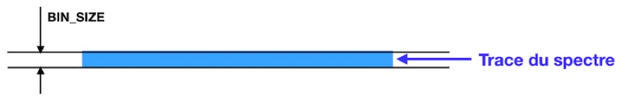
BIN_SIZE : Mandatory parameter. Width in pixels of the binning (or agglomeration) area of the 2D spectrum along the spatial axis to build the spectral profile. It is recommended that this width allows to encompass most of the signal of the object along the spatial axis (vertical), say 99% of this signal to avoid photometric errors. An excessive width for the binning area may result in added noise (to a lesser extent if the value of the optional parameter extract_mode is 1.)
Example :
bin_size: 24
CALIB_COEF : This parameter is mandatory if the « calib_mode » parameter takes the values 1, 2 and 4. Terms of the spectral dispersion polynomial as a list starting with the highest degree term, e.g. [A4, A3, A2, A1, A0]. specINTI evaluate the degree of the polynomial from the number of terms provided.
Example:
calib_coef: [-4.82275e-10, 4.5412e-6, 0.96946, 3771.874]
CALIB_MODE : Optional parameter. Selection of the spectral calibration mode according to the value of the parameter.
If the value is 0 : classical calibration with a spectrum of emission lines from a reference lamp. specINTI calculates the dispersion polynomial with these lines. This is the default mode.
If the value is 1 : the calibration is performed using only the terms of a predefined dispersion polynomial, which has been entered (calib_coef parameter).
If the value is 2 : the calibration is made from the terms of a predefined dispersion polynomial, which has been entered elsewhere (calib_coef parameter), but in addition the software uses the emission lines of a standard lamp spectrum to precisely calibrate the spectrum in translation only.
If the value is 3: the calibration is performed in lateral mode using the emission lines of a reference lamp spectrum turned on during the exposure time of the target. The dispersion polynomial is evaluated from the emission lines.
If the value is 4: the calibration is performed using the terms of a predefined dispersion polynomial, which is indicated elsewhere (calib_coef parameter), but whose first term (translation) is adjusted using the emission spectrum of a lateral reference spectrum superimposed on the target spectrum.
The parameter can also take on negative values for special modes - see Sections 6 and 7 for details.
Example:
calib_mode: 2
CLEAN_WAVE : Optional parameter. A list of wavelengths around which the software performs a linear interpellation on a width provided in the corresponding clean_wide parameter. This function allows to erase some artifacts or telluric lines identified by their wavelength in angstroms.
Example :
clean_wave: [6543.9, 6552.5]
CLEAN_WIDE : Optional parameter. A list of spectral widths in angstroms at the ends of which the software performs a linear interpellation to clear a detail of the processed spectral profile. This parameter is used in conjunction with the clean_wave parameter.
Example :
clean_wave: [2.0, 2.4]
CORR_ATMO : Optional parameter. If this parameter is present, the software calculates the non-molecular atmospheric transmission and applies it to the processed spectrum in order to find an off-atmosphere profile. The parameter is the AOD value (aerosol transparency of the atmosphere). Recall that very dry mountain air has an AOD of 0.02 and for a dry desert the AOD is 0.04. In France, the AOD is 0.07 in winter, 0.21 in summer, and on average over the year 0.13. When the weather is very hot and stormy, the AOD can reach 0.50. For our observation, made in summer, near the sea, but not on a properly transparent night, we adopt the average value: AOD = 0.13.
The equatorial coordinates of the object are essential for the calculation of the angular height of the object in relation to the horizon line. Normally, these coordinates are found in the file header, through the CRVAL1 and CRVAL2 keys. If these keys are not defined, then the calculation is not continued, unless the search for these coordinates in the SIMBAD database is implicitly requested via an Internet query. There are three conditions for this: (1) that the « simbad » parameter with the value 1 is present in the configuration file, (2) that there is an open Internet connection, (3) that the object name is recognized in the SIMBAD database. The search for equatorial coordinates is then automatic and transparent. Finally, we remind you that it is possible, in case of force majeure, to define the CRVAL1 and CRVAL2 keys manually thanks to the function process in the configuration file (function «_img_add_item_float »)
Example :
simbad: 1
corr_atmo: 0.13
CORR_ATMO2 : Optional parameter. Similar in its function to « corr_atmo », this one has two arguments, in order, the value of the AOD, then the value of the angular height of the star in degrees. In other words, it is no longer necessary to provide the equatorial coordinates of the star, nor the geographic coordinates, but you must have established the angular elevation of it elsewhere.
Example :
corr_atmo2: [0.13, 42.7]
CORR_TOPO : Optional parameter. If this parameter is present, the software calculates the topocentric radial velocity of the observer towards the object. The calculation takes into account the geographical coordinates of the observer on the surface of the Earth (the parameters longitude, latitude and altitude become mandatory), and of course the rotation of the Earth around the Sun. The internal precision of the calculation is of the order of a centimeter per second (it is therefore very accurate).
Moreover, the value of the parameter is the proper radial velocity of the object in km/s (this information is retrieved from databases, like SIMBAD, but must be provided implicitly). If the object's own radial velocity is not known, enter the value 0. According to the standard in SIMBAD, if the object is moving away, the radial velocity is positive and in the opposite case, it is negative.
In our definition, the global radial velocity calculated (topocentric velocity plus proper radial velocity) is positive if the object is moving away from the Earth and negative if it is approaching it.
In a second step the software corrects the wavelengths of the spectrum to bring it back to an object at rest ("rest wavelength").
The equatorial coordinates of the object are essential for the calculation of the topocentric velocity. Normally, these coordinates are found in the header of the files, through the keys CRVAL1 and CRVAL2. If these keys are not defined, then the calculation is not continued, unless the search for these coordinates in the SIMBAD database is implicitly requested via an Internet query. There are three conditions for this: (1) that the « simbad » parameter with the value 1 is present in the configuration file, (2) that there is an open Internet connection, (3) that the object name is recognized in the SIMBAD database. The search for equatorial coordinates is then automatic and transparent. Finally, we remind you that it is possible, in case of force majeure, to define the CRVAL1 and CRVAL2 keys manually thanks to the function process in the configuration file (function « _img_add_item_float »)
Example :
simbad: 1
corr_topo: -12.45
COSMIC_TH : Optional parameter. Advanced parameter acting on the cosmic ray detection threshold when the optimal extraction of the profile is requested (see the extract_mode parameter). The default value is 25, and should not be changed, except to spot artifacts in the spectral profile when optimal extraction is requested.
Example :
cosmic_th: 50
CROP_WAVE: Optional parameter. Isolates a portion of the final calculated spectrum, portion delimited by two wavelengths: [lambda1, lambda2]. This parameter helps, for example, to extract the part of the spectrum considered significant.
Example :
crop_wave: [3800, 7500]
EXPAND : Optional parameter. If this parameter is defined, at the end of the processing, specINTI generates a new 2D image, representing the spectral profile expanded along the vertical axis on the number of lines passed in parameter (the profile is duplicated x times). There are in fact two images produced, in FITS format and in PNG format.
Example :
expand: 800
EXTRACT_MODE : Optional parameter. If the value is null (default value), specINTI extracts the raw spectral profile from the 2D spectral images by performing a simple column-by-column addition in the bin_size width. This is an expedient method that is suitable for bright objects. If the signal of the spectrum is very weak compared to the noise, it is better to use an optimal extraction method that significantly reduces the noise in the profile by performing a weighted addition. The algorithm also removes cosmic rays that may be in the binning area in an iterative process (Keith Horne ,1986; "An Optimal Extraction Algorithm for CCD Spectroscopy", PASP v. 98, p. 609). We activate the optimal extraction by giving the value 1 to the parameter.
Attention, if the optimal extraction is requested, the parameters noise and gain become mandatory.
Example :
extract_mode: 1
noise: 2.5
gain: 0.042
Another dependent parameter is « cosmic_th ».
FIT_ORDER : Mandatory parameter in mode -4. Order of the polynomial adjusted with the special mode -4.
Example :
fit_order: 800
FIT_POSX : Mandatory parameter in mode -4. List of line positions in pixels, operated with the special mode -4 (the typical application is the manual calculation of a spectral dispersion polynomial).
Example :
fit_posx: [307, 369, 508]
FIT_WAVELENGTH : Mandatory parameter in mode -4. List of wavelengths, operated with the special mode -4 (the typical application is the manual calculation of a spectral dispersion polynomial).
Example :
fit_wavelength: [3948.979, 4044.418, 4259.362]
FLAT_MODE : Optional parameter. This is an advanced parameter, related to the optimal extraction of the profile (optimal binning, see the extract_mode parameter). The default value is 0, and corresponds to a standard usage of the flat-field image. In this situation, the flat-field correction is performed on the raw images. However, this can change the distribution of noise in the sky background as a function of wavelength, which will disturb the optimal extraction algorithm (only in the situation of spectrography at low spectral resolution in general). If the value of the extract_mode parameter is 1, it may be useful to perform the flat-field correction at the final profile level by assigning the value 1 to the flat_mode parameter. The result of the correction is less rigorous in terms of bias correction, but may be more favorable in terms of noise reduction for very weak objects (to be tested according to the circumstances). Generally we use the value 0, which is also the default value if the parameter is not defined.
Example :
flat_mode: 1
GAIN : Optional parameter, unless extract_mode = 1. Electronic gain of the camera in electrons / ADU.
Example:
gain: 0.042
HOT_PIXELS : Optional parameter. Eliminates the hot pixels in the image of the dark signal. A pixel is considered hot if its intensity exceeds the value given in the parameter, expressed in ADU. The intensity of the pixel is replaced by the average of the intensity of its 8 neighbors.
Example:
hot_pixels: 6500
HOT_PIXELS2 : Optional parameter. Eliminates the hot pixels in each image of the spectrum of a sequence. A pixel is considered to be hot if its intensity exceeds the value given in the parameter, expressed in ADU units. The intensity of the pixel is replaced by the average of the intensity of its 8 neighbors.
Exemple:
hot_pixels2: 50000
INSTRUMENTAL_RESPONSE : Optional parameter. Name of a FITS file, of the spectral profile type, containing the instrumental response of the instrumental set (the telescope, the spectrograph, the detector). This file must be located in the directory of the processed session (working folder). As soon as the parameter is used, the extracted spectrum is corrected for the instrumental response.
Example :
instrumental_response: reponse_starex300
KERNEL_SIZE : Optional parameter. specINTI offers the possibility to apply a median filter to the 23D images before extracting the spectral profile. This filter is particularly useful with CMOS sensors where impulse noise is present (called telegraph noise, or RTS, or "salt and pepper"). The value of the parameter is the size of the convolution kernel. An odd value must be provided. For example the value 3 corresponds to a convolution kernel of 3x3 pixels. It is not recommended to exceed the value 5.
If you provide a negative value, the software still performs a median filtering, but with an optimized weighting algorithm, both effective on the impulse noise, but restoring places the details of the image than a classic median filtering. Note that the optimal algorithm is slower to execute than the standard algorithm.
Example :
kernel_size: -3
LINE_POS : This parameter is mandatory for some calibration modes. It specifies the coordinates in pixels in the image of the spectrum, along the spectral axis, of lines whose wavelengths are also provided with the wavelength parameter. If the calibration lines are well tilted (slant) make sure to perform the measurement of the positions at the intersection with the spectrum trace. For example :
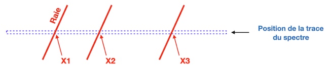
Don't worry too much about the accuracy of these readings. By default, the error can be +/-25 pixels. You can change the value of this uncertainty range using the search_wide parameter (reduce or increase it).
Example :
line_pos: [237, 450, 633]
NOISE : Optional parameter, unless extract_mode = 1. Provides the software with the value of the electron detector reading noise.
Example :
noise: 2.5
NORM_WAVE : Optional parameter. If this parameter is defined in the configuration file, the final spectrum is normalized to unity using the average of the intensities included in a spectral region determined by two wavelengths provided in parameter [lambda1, lambda2].
Example :
norm_wave: [6600, 6620]
PLANCK : Optional parameter. If this parameter is defined in the configuration file, the final spectrum is multiplied by the Planck profile calculated for the temperature in degree K provided in parameter.
Example :
planck: 2900
POLY_ORDER : Mandatory parameter if calib_mode is 0, 3 or -1. Fix the order of the dispersion polynomial found from the lines of a calibration lamp. If n is the number of lines used, the order of the polynomial cannot be higher than n-1.
Example :
poly_order: 3
POSY : Optional parameter. Normally, specINTI calculates a vertical coordinate (along the Y axis) of the spectrum trace specific to each image of a sequence. The processing is somehow individualized for each image, for an optimal result. But there may be situations where the trace is almost imperceptible or where you do not want the software to do the calculation for you (processing the spectrum of nebulae for example). In this last situation, define the posy parameter in the configuration file by specifying the Y-coordinate of the spectrum. specINTI then takes as a base the indicated vertical coordinate of the trace for all images of the sequence.
If the posy value is negative, the software considers that the spectrum trace is vertically located approximately at the indicated Y coordinate (in absolute value), but in addition, it recenters all spectra within the binning limit (bin_size parameter). The posy parameter with a negative value is a powerful tool that allows to get out of complex situations such as extracting the spectrum of a weak object whose trace is located near that of a much more intense object.
Be careful not to generalize the use of posy. The use must be a case of force majeure, because the calculation made by specINTI will always be more accurate. In the overwhelming majority of situations, the software automatically finds the correct value for the position of the spectrum trace, so you should not use the posy command.
Example:
posy: 376
POSY_EXCLUDE : Optional parameter. Defines an exclusion zone for the calculation of the vertical Y coordinate of a spectrum trace. The argument of this parameter is a pair of coordinates (Y1, Y2) that delimits a band inside which the search is performed. Areas of the image outside this band are not used. The posy_exclude parameter is of interest in particular applications where parts of the spectrum may interfere with the search for the spectrum trace. This is for example the case when a photometric slit is used, whose widened part can be a source of difficulty.
Example:
posy_exclude: [250, 600]
RATIO : Optional parameter. If the value of this parameter is 1, at the end of processing, the ratio of the spectrum of the first two objects provided in the "Object list" of the observation file is calculated. The result is a profile file in the working directory, with the name of the profile of the first spectrum, to which is added the text "_ratio".
The calculation is ignored if there is only one object in the "Object list". The default value is 0 (the ratio calculation is not performed).
Example:
ratio: 1
SEARCH_WIDE : Optional parameter. Modifies the tolerance on the value of the horizontal coordinates of the lines indicated with the line_pos parameter. By default the uncertainty is +/-25 pixels, which corresponds to a parameter value of 50. If necessary, you can increase the value if the calibration lines are well separated from each other and on the contrary reduce it if the lines are close and if there is a risk that they will be confused by the software.
Example :
search_wide: 68
SHIFT_POSX : Optional paramètre. . Décale Shift all the element of POSX or FIT_POSX table by the given value.
Example :
shift_posx: -10
SIGMA_GAUSS : Optional parameter. Application of a Gaussian filtering to the 2D images of the spectrum if the value of the parameter is not null. The higher the value, the more the filtering is supported. This smoothing reduces the noise, but can lead to a reduction of the final resolving power. A value between 0.5 and 1.5 is typical (it should be tested to find the best compromise between noise reduction and reduction of the fineness of the spectra).
Example :
sigma_gauss: 1.0
SNR : Optional parameter. Returns in the output console the signal to noise ratio (SNR) after processing a spectrum. The calculation area in the processed spectral profile is included in lamb1 and lamb2 (in angstroms). Ideally, the area of calculation thus defined must be located in the continuum of the spectrum, in a part without spectral lines. Before calculating the noise, necessary for the evaluation of the signal-to-noise ratio, specINTI removes the best straight line passing through all the points of the area in order to reduce the bias induced by a slow variation of the spectral profile in the area.
Example:
snr: [6550, 6560]
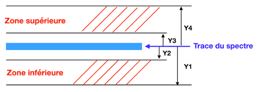
SKY : Mandatory parameter. Set of coordinates in pixels along the spatial axis (vertical) delimiting two areas of calculation of the sky background signal on either side of the spectrum trace. These coordinates are relative to the vertical coordinate of the spectrum trace. The format of the parameter data is [y1, y2, y3, Y3], with the following geometric interpretation (values are always in absolute):
Example:
sky: [180, 30, 30, 180]
The indicated coordinates can be perfectly asymmetrical with respect to the spectrum trace, for example :
sky: [110, 25, 30, 180]
The values of the coordinates provided must be defined carefully, because they are used many times in specINTI, not only to calculate the sky background. The coordinates (y2, y3) define an area in which an optimal filtering is requested (see the kernel_size parameter). The coordinates y1 and y4 are also used to evaluate the slant angle of the lines (a geometrical defect, see also the slant parameter).
Note that specINTI does not use default values to define the size and position of the sky background calculation areas because the user's judgment is important here. These zones must first exclude the processed spectrum trace. On the other hand, an excessive width may cause residual errors in the geometric correction of the spectrum to affect the final spectral profile, or may result in accidental blending with the trace of a nearby object. You should also not go outside the boundaries of the image (specINTI will tell you if this is the case). A width that is too narrow can generate noise because then you average few pixels column by column --- no averaging effect then. A calculation height of 100 to 250 pixels is generally considered correct. In general, the sky parameter values never change for a given instrumentation.
SKY_MODE : Optional parameter. Choice of the method used to remove the sky background (see also sky parameter). If the parameter is 0 (default value), for each column independently, the software calculates the median intensity in the sky background evaluation areas and subtracts this value from the column. If the parameter is 1, the software fits a Legendre polynomial through the intensity of the sky background in the evaluation areas, then subtracts the interpolated value from the spectrum trace along the column in question. The latter technique is generally more accurate, but also slower in execution time.
Example :
sky_mode: 1
SKY_REMOVE : Optional parameter. If the value is 0, the sky background is not removed from the images (useful for some nebula observations for example). If the value is 1 (default value, almost always adopted), the sky background is removed (see sky_mode parameter).
Example :
sky_remove: 1
SLANT : Optional parameter. Normally, the slant angle of the spectral lines is determined automatically by specINTI :
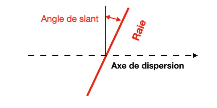
The software uses this angle to straighten the lines so that they are vertical. You can however impose the value of the slant angle through the « slant » parameter, by providing the value of this angle (in degrees).
Example :
Slant: -0.51
SMILE_RADIUS : Optional parameter. The smile is a geometric deformation of the spectral lines, which instead of being straight have a curved shape, with a radius of curvature R in pixels, which is the value of the parameter :
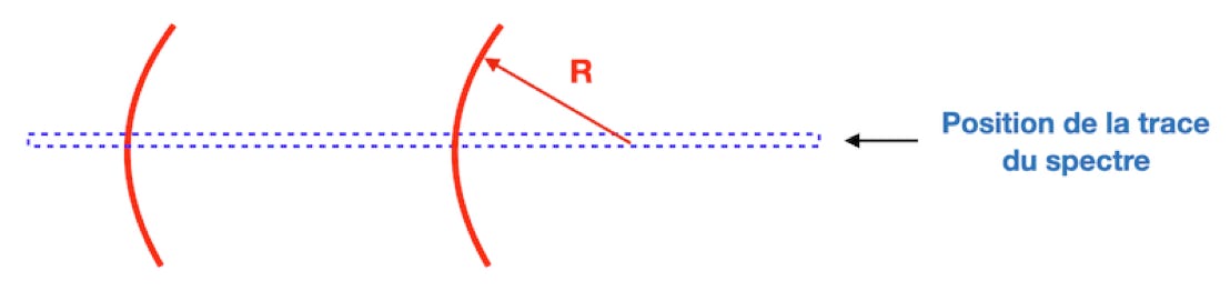
The smile is specific to some categories of spectrographs only. When the radius of curvature of the lines is defined through the smile_radius parameter, specINTI corrects the distortion in the 2D images so that the lines are straight in the end.
A tip: if the check_mode parameter is 1, the software produces in the working directory an image _step5.fits which shows the shape of the calibration lines before correction of the smile effect, and the image _step71.fits after correction.
Example :
smile_radius: -18500
SPECTRAL_SHIFT_WAVE : Optional parameter. Spectral shift of the final profile by a certain amount in angstroms. Can correct a systematic calibration error, for example.
Example:
spectral_shift_wave: 0.24
SPECTRAL_SHIFT_VEL : Optional parameter. Spectral shift of the final spectral profile by a certain amount in km/s. Can correct a Doppler shift, for example.
Example :
spectral_shift_vel: -22.3
TILT: Optional parameter. Normally, the tilt angle of the spectrum trace is determined automatically by the specINTI :

The software uses this angle to take the horizontal trace (which is recommended during acquisition). You can however impose the value of the tilt angle through the tilt parameter, by providing the angle in degrees.
Example :
tilt: -1.32
XLIMIT : Mandatory parameter. Set of two values in pixels delimiting a region of the trace in which the software will perform a number of calculations to extract the spectral profile. The format is [x1, x2], with x1 and x2 the limits which frame a part of the spectrum trace judged as sufficiently intense for the calculations to proceed correctly. The choice is very flexible. Let's just say that the trace must be perceptible and of a relatively constant width. Typically the value of x2 - x1 must be greater than 200 pixels, but can very well be 2000 pixels.
Example:
xlimit: [452, 1966]
WAVELENGTH : Mandatory parameter for some calibration mode. A set of calibration line wavelengths that allow specINTI to compute the dispersion polynomial (relationship between the rank of pixels along the spectral axis in your images and the wavelengths).
This parameter is closely related to the line_pos parameter, which specifies the approximate positions of the corresponding lines in your 2D images.
You can perfectly specify a single line or a list of very many lines. Examples :
wavelength: [6532.88]
wavelength: [6506.53, 6532.88, 6598.95, 6678.28]
WIDE_SOURCE : Optional parameter. If the value of this parameter is 1, specINTI enters a simplified mode of calculation as soon as the object has a large surface (in particular, the sky background parameters are not required). See the Lab'Ex application appendix for more details on the use. The default value of the parameter is 0.
Example :
wide_source: 1
12.3 : Exploitation parameters
ALTITUDE : Optional parameter. Altitude of the observation site in meters. This information is written in the header of the FITS file of the processed spectrum.
Example :
altitude: 105
CHECK_MODE : Optional parameter. This parameter determines the nature of the outputs on the screen (console) or in the working directory during the processing. If the value is 0 (default value), the information delivered is limited to what is necessary. If the value is 1, specINTI provides more information about each processing step and writes image and spectrum files corresponding to these steps into the working directory (files with reserved names _stepxxx and _profilexxx). Option 1 is particularly useful for checking the correct processing and for spotting errors and for troubleshooting users in difficulty (a kind of after-sales service!).
Example :
check_mode: 1
FILE_EXTENSION : Optional parameter. Choice of extension type for FITS files. If the value is 0 (default value), the extension is ".fits". If the value is 1, the extension is ".fit".
Example :
file_extension: 1
INST : Optional parameter. Title of the observation material. This information is written in the header of the FITS file of the processed spectrum.
Example :
inst: T250+Solex(300)+ASI183MM
LATITUDE : Optional parameter. Latitude of the observation location in degrees. This information is written in the header of the FITS file of the processed spectrum.
Example :
latitude: 34.5701
LONGITUDE : Optional parameter. Longitude of the observation location in degrees. This information is written in the FITS file header of the processed spectrum.
Example :
longitude: -1.4677
MASTER_PATH: Optional parameter. Specifies the path to a directory containing DOFs with a name beginning with "__". Images from this location are used if in specINTI they are also designated by "__".
Example :
master_path: d:/my_master/
NEAR_STAR : Optional parameter. Name of an object located near the target under study. If this parameter is defined, then specINTI uses the name of the object provided as a parameter to compute the equatorial coordinates of observation rather than the catalog name provided in the observation file. This is useful when the target has a name that is not recognized by SIMBAD (asteroid, nova, etc), because you can still correct the atmospheric transmission data and the topocentric velocity correctly, as the object is close in the sky.
Example :
near_star: SAO 16325
POWER_RES : Optional parameter, mandatory only if calib_mode = 1. This information is written in the header of the FITS file of the processed spectrum.
Example :
power_ref: 15000
SEQ_MODE : Optional parameter. Writes the individual processed spectra of a sequence to your disk in the working folder. Files name are @object-xxx is the parameter value is 1 and _@object_YYYYMMDD_FFFFF if the value is 2.
Example :
seq_mode: 1
OBSERVER : Optional parameter. Name of the observer. This information is written in the header of the FITS file of the processed spectrum.
Example :
observer: C. Buil
SITE : Optional parameter. Name of the observation site. This information is written in the header of the FITS file of the processed spectrum.
Example :
site: Antibes St Jean
VERSION : Optional parameter. Returns the version of the specINTI software if the parameter value is 1. The execution of the program stops after the version number is displayed.
Example :
version: 1
15 : Functions Reference Manual
Functions are one-line commands that are inserted into the configuration file. When such a function is present (its name begins with the character "_"), its associated code is executed, then the program stops.
_version:
Return the specINTI current version.
_img_add: [in1, in2, out]
Adds the images (in1) and (in2) with the result (out).
_img_add_item_float: [in, item, value, out]
Adds an item of type (float) to the header of a FITS image.
_img_add_item_int: : [in, item, value, out]
Adds an item of type (int) to the header of a FITS image.
_img_add_item_str: : [in, item, value, out]
Adds an item of type (string) to the header of a FITS image.
_img_compute_smile: [x1, y1, x2, y2, x3, y3]
Calculates the radius of curvature and center of a circle from the coordinates of 3 points on the circle. This function is useful for determining the radius of curvature of a line (whose shape is assimilated to a circle) so as to correct this distortion and make the line straight (i.e. with an infinite radius of curvature). The result is displayed in the output console. Example:
_imag_compute_smile: [1669, 23, 1666, 414, 1669, 678], resulting in a radius of curvature of 17200 pixels.
_img_fill: [in1, x1, x2, out]
Zeros the parts of the image (in) between x=1 and x=x1 on the one hand, and between x=x2 and x=max width on the other. The result is the image (out).
_img_make_offset: [in, out]
Generates an image (out) whose intensity is equal to the average of the intensities in the image (in).
_img_merge: [in1, in2, threshold, out]
Merge of two images exposed briefly (in1) and long (in2) by the HDR technique. The threshold defines the saturation level in the image (in2).
_img_offset: [in, offset, out]
Adds a constant (offset) to the image (in). The result is the image (out).
_img_sub: [in1, in2, out]
Calculates the difference between the images (in1) and (in2). The result is the image (out).
_img_uniform: [in, value, out]
Generates the image (out) of the same format as the image (in) with the intensity of all pixels equal to (value).
_img_smile: [in, radius, y0, out]
Applies a "smile" type distortion to an image, with the radius of curvature (radius, in pixels) and y0, the height of the center of curvature (in pixels).
_pro_blur: [in, coef, out]
Filters a profile with the SAVGOL algorithm with a strength adjusted by the value (coef).
_pro_clean: [in, w1, w2, out]
Linear interpolation between wavelengths w1 and w2. You can perform this function several times by writing _pro_clean1, _pro_clean2, ...
_pro_div: [in1, in2, out]
Divides the profile (in1) by the profile (in2) with the result (out).
_pro_conv_melchiors: [in, in, telluric]
Converting a FITS spectrum from the Melchiors library into a simplified FITS profile. If telluric = 0, the Melchiors spectrum version is cleaned of telluric lines, if telluric = 1, telluric lines are present.
_pro_fit: [in, w1, w2, w3, w4, out]
Smoothing of the profile (in1) by a parabolic function passing through the wavelengths w1, w2, w3, w4 (in A) at best. The smoothed result is the profile (out).
_pro_fit2: [in, w1, w2, w3, w4, w5, out]
Smoothing of the profile (in1) by a polynomial function of degree 3 passing through wavelengths 5 wavelengths at best.
_pro_fit3: [in, w1, w2, w3, w4, w5, w6, out]
Smoothing of the profile (in1) by a polynomial function of degree 3 passing through wavelengths 6 wavelengths at best.
_pro_gauss: [in, sigma, out]
Convolution of the profile (in) by a gauss function, width (sigma, in A). The result is the profile (out).
_pro_norm: [in, w1, w2, out]
Normalizes the input profile to unity using the average found between the wavelengths (w1) and (w2). The result is the (out) profile.
_pro_offset: [in, offset, out]
Adds a constant (offset) to the profile (in). The result is the profile (out).
_pro_shift_vel: [in, v, out]
Applies a spectral shift in velocity (v, in km/s) to all points of the profile (in) to produce the profile (out).
_pro_shift_wave: [in, w, out]
Applies a spectral shift in wavelength (w, in A) to all points of the profile (in) to produce the profile (out).
_pro_snr: [in, lamb1, lamb2]
Returns in the output console the signal to noise ratio (SNR) of the spectral profile (in), calculated between the lamb1 and Lamb2 terminals in ansgtröms.
_pro_telluric: [atmo, in, out]
Removes telluric lines from a spectrum. [atmo ] is the name of a FITS file of the molecular spectrum of the Earth's atmosphere. It is a synthetic spectrum, among those contained in the "atmo_molecular" archive, whose data is a spectrum shaping from the ESO Sky Model Calculator. [in] is the name of the starting spectral profile, and [out] is the same profile after the removal of telluric lines. This function also writes in the working directory the @atmo spectrum of the atmosphere fitted in the least squares sense to the observed spectrum. For application examples see section 5.8.4 and A4.3
16 : Ressources
Sol’Ex/Star’Ex site : http://www.astrosurf.com/solex/
YouTube : Astro-Spectro
Sol’Ex/Star’Ex on Facebook
Sol’Ex list : https://groups.io/g/Solex-project
« Spectrographie, détecteurs et astronomie » site : http://www.astrosurf.com/buil/index.html
A two-part presentation introducing the use of specINTI, based on observations made with a 100 mm diameter telescope in high spectral resolution:
Vidéo #1
Vidéo #2

In the form of a PDF file, a presentation given at the Star'Ex workshop on January 21, 2022, with lots of tips and an introduction to specIINTI : bien_débuter_avec_starex.pdf
In the form of a PDF file, a presentation given at the Star'Ex workshop on January 21, 2022 (in French), with lots of tips and an introduction to specIINTI :