We have 8 spectra of the Be star HD192685. They are each 300 seconds exposure. We will use the same master images as for the star Altair.

The images have the generic name "192685-". Download the images: 192685.zip (740 KB)

A remark about how to organise the file images. First, we use a directory per night (The name is generated from the day, month and year. For example 130606 for June 13, 2006). The objects in this folder are identified by their name, here the HD number. To separate the catalogue number of the object and the serial number of the image, a dash is always inserted between the two. Our images on the disk have the names 192685-1.pic, 192685-2.pic, 192685-3.pic, ...

Run the command:

> number  192685-

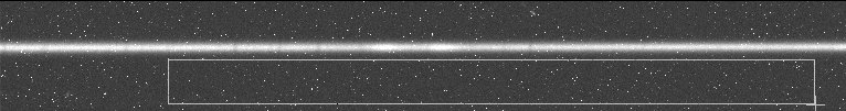
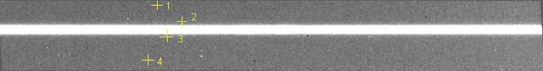
Use the mouse to select the area where the thermal noise compensation will be carried out:

Open the basic pretreatment dialog box (Spectro menu):

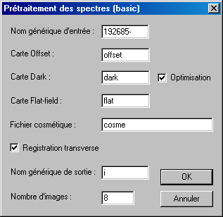
Normally all fields are pre-filled. Just click OK.

At the end of the calculation, SPiris returns the angle of tilt of the spectrum (here -0.041 °).

Ignore the spectrum displayed on the screen, which is a simple arithmetic sum of the 8 individual spectra. We will calculate an optimal addition of the pre-processed images i1, i2, ... I8 elliminating the few cosmetic defects. Open the dialog box Add a sequence from the Treatment menu.

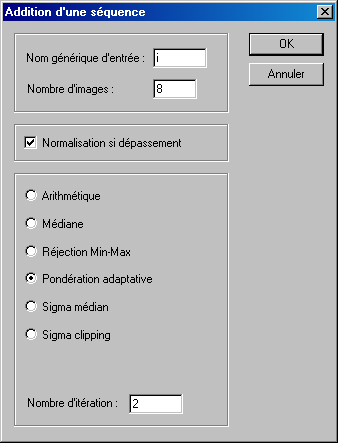
Choose the adaptive weighting option, then click OK. The result:

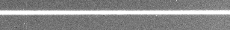
Make the geometric correction:

> slant  50  -3.5
> tilt  380  -0,041

Run the command

>l_sky2

Then select 4 points to define the sky background:

The result is the level 0b product

>save t192285_1

The level 0b spectrum of the star HD192285.

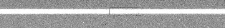
To calculate the 1D profile using the command l_opt first select the spectrum with the mouse:

Then we do

>l_opt

The level 0c spectrum of the star HD192285.

>save t192285_2

>l_plot

The processing of the 2D data has been completed. You can go to the next star!

5.5. Processing the spectrum of the star 55 Cyg

We have 10 spectra of the Be star 55 Cyg. 300 seconds exposure each.

Download images: 55cyg.zip (900 KB)

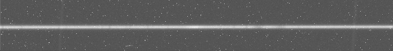
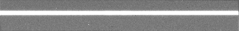
A raw spectrum of the 55 Cyg sequence.

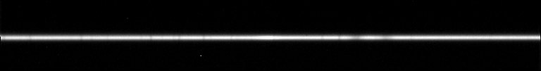
The level 0b spectrum of 55 Cyg.

The level 0c spectrum of 55 Cyg.

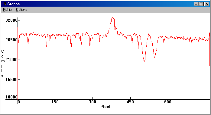
The uncalibrated spectral profile (level 1a product). Both lines to the right of Halpha
Are due to CrII located at wavelengths A 6578.03 and 6582.85.

To see the results, you can:

-- download image t55cyg_1
-- download image t55cyg_2

5.6. Processing the Delta Sco spectrum

We have 9 spectra of the Be star Delta Sco, each 300 seconds exposure (dsco-1, dsco-2, ...).

Download the images: dsco.zip (860 KB)

Here is the result of the processing:

The level 0b product.

Viewing the level 1a product in graphical form.

5.7. Calculation of a level 1b product

One of the great strengths of the fully automatic processing tools seen in sections 3 and 4 is that they allow an accurate spectral calibration to be made easily. This calibration is of course feasible in "manual" mode too using the individual commands.

Remember that a level 1a product is an ASCII file in which the spectral line is represented by pixel values:

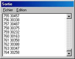
A file spectrum 1a.

The purpose of the spectral calibration is to move from a level 1a product to a level 1b product. Remember that the dispersion law of a level 1b product is linear. To achieve this, we must apply a second (possibly third) order polynomial function of wavelength to the level 1a product. The result is a 1-D, two column file: the wavelengths are in the first column, the corresponding intensities are in the second column.

The command l_calib2 uses the positions of water vapour telluric lines to perform the calibration. Atmospheric lines are more intense in the Halpha area. Warning, this command only works with spectra centred approximately on the the Ha line using the LHIRES III, with a 2400 l / mm grating. It is of course also important that the telluric lines are visible with good contrast (This is almost always the case in the summer season provided the star is not too faint). The command l_calib2 is used by the dialog box Treatment spectra LHIRES III - 2400 during the spectral calibration.

the wavelengths of the lines used (angstroms) are:

6532,359
6543,907
6548,622
6552,629
6572,086
6574,852
6580,785
6586,570

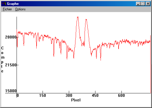
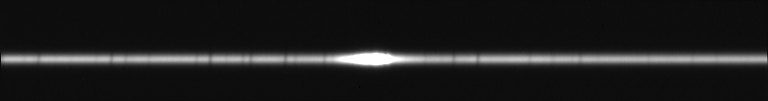
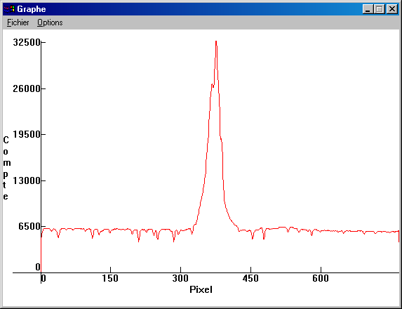
The software automatically performs an adjustment using a second order polynomial. The software identifies the position of the telluric lines for you. The polynomial coefficients are returned and a level 1b spectrum is created in the working directory. Two parameters are needed to produce the level 1b spectrum. The filename (SPiris adds the extension. Dat to the filename), and the approximate position in pixels along horizontal of one of the telluric lines. The line in question is at the wavelength 6574,852 A. It is distinct and easy to identify unambiguously. It is shown in the spectrum below:

Locating the line H2O to 6574,852 angstroms.

In our example of the Altair spectrum, the line is located approximately at the coordinate x = 480. Use the mouse pointer to find this value. It need not be precise, even if you make a mistake of 3 or 4 pixels, the software can still work accurately.

Load spectrum level 0c (1-D spectrum duplicated 20 times in verical axis):

> load taltair_2

Then run the command:

> l_calib2 taltair_3 480

Note: the command l_calib also exists, but it only applies to spectra acquired with the 1200 l / mm grating. It uses neon lines to perform the spectral calibration. l_calib2 do not need these (the latter uses only the position of the telluric lines).

The file taltair_3.dat is written to disk. The image in memory is also re-interpollated to linearize it. Now, an interval of 1 pixel along the spectrum axis represents a 0.11570 angtrom step.

The Output window gives the result of the calculation:

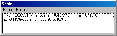
Spectral calibration parameters.

The parameters a0, a1, a2 are the polynomial coefficients found based on the telluric lines. In the raw spectra, if x is the position of a pixel, we have the relationship:

The coefficients a1 and a2 are almost constant for a given instrument. They can be used in VisualSpec to produce non-linear spectral calibrations, even when there are no marked telluric lines (eg the star is too faint).

The RMS value is the error in angstroms of the calibration points compared to the real spectrum. Here the difference is 0.0077 angstrom, equivalent to a velocity of approximately 350 meters/second. This is very precise, which shows the quality of the methodology used (there is no human intervention to measure the position of the lines, which greatly reduces the risk of errors and improves the consistency of the method). On the other hand, if you find an RMS error of a few tenths of angstroms, you have probably made a mistake (often a misidentification of the H2O line at 6574 angstroms).

Here is the content of the spectrum taltair_3.dat

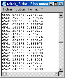
Extract 1b spectrum

The level 1b spectrum can be imported into VisualSpec (with the load dat file option) and can be corrected photometrically (division by the instrument's response, normalization to the continuum, ...), and analyzed.

<previous>    <summary>    <next>    Page 4 / 6