Mouse Wheel 
Visual Spec is now
responding to mouse wheel in the two following cases:
Open an image, click in the image and
use the mouse wheel to reduce or enlarge the thresholds window. A
reduced window width will increase the contrast.
Open a profile, click on the profile
at the position you want to keep centered. Use the mouse wheel to zoom around
this position. you can always revert to the original display with the
"unzoom" button. if no profile position has been indicated (by a
simple click) the zoom will be centered on the middle of the profile.
|
Display Positions next to cursor
If you want to have the
display of the X, Y position of the cursor next to it, click on the
small square next to the X,Y label in the toolbar.
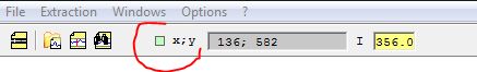
If the mouse is over an
image, it will display the X,Y coorinates.

If the mouse is over a
spectrum profile, it will display the pixel and its wavelength. The
wavelength is zero if the profile is not calibrated.

|
Image sky background subtraction
If you want to subtract
the sky background above and below the spectrum, there is now a new button in
the toolbar

A new dialog box will be
displayed
The algorithm can find
automatically the spectrum if there is only one spectrum in the image. But if
you un-select the Auto mode, enter the Y position of the middle of the
spectrum in the image.

The sky background
correction compute a column by column average value from two regions above
and below the spectrum region. The width of those windows can be
modified. This profile can be assimilated to the sky spectrum and is then
subtracted as an offset to the entire image.
If the auto mode is
selected, Visual Spec will pick two sky regions at 10 pixels above and below
the profile region.
If the auto mode is unselect, enter the Y top and bottom coordinates of the
two prefered regions.
|
Image raw profile extraction
This function extract and
display the profile of the spectrum from one image. Go in the menu
Extraction>Basic profile extraction.

The dialog box is similar
to the sky subtraction box. The two additional functions are the tilt
correction and the binning profile extraction. If the tilt angle mode is
selected, Visual Spec will compute the rotation angle along the horizontal
axis. The value found will be set in the text field next to it. If
unselected the text field is active and the angle value will be the one
entered in the text field.
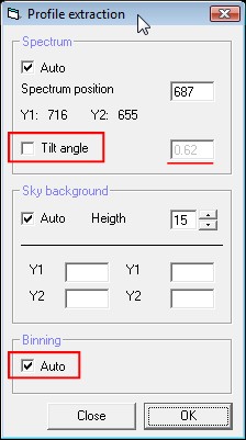
The binning auto mode
will use the specific binning algorithm of Visual spec which retains only
lines which contains signal. If the auto mode is unselected, a classic sum is
made column by column in the region around the spectrum defines at the
beginning of this process.
The raw profile is
displayed in a profile document. The resulting profile is the spectral
profile, but not yet calibrated. The tilt angle is corrected, but not the
slant, as this is not necessary for a such basic function.
|
Image basic calibrated profile extraction
This function extracts,
calibrates and displays the profile of the spectrum from one image. It is
based on the above described steps in the raw profile extraction with the
addition of a set of field to perform a basic calibration.
Go in the menu
Extraction>Basic profile extraction.

A dialog box is opened.
On the left, the panels have the same function as in the function above. The
right panel is for the basic calibration of the raw profile. To perform a
very basic calibration you need to identify 2 lines and assign the
wavelength to the pixel positions.

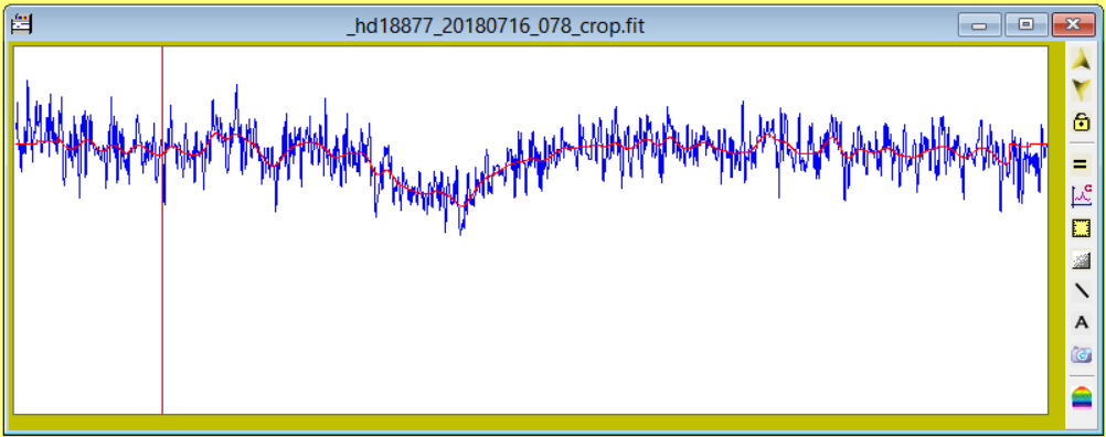
If you turn on the
display X,Y position next to the cursor, you can move it on the image and see
where are the lines. In the exemple above, the H-alpha line at 6563 is
visible as an absorbtion line, and the first O2 atmospheric molecular
absorbtion band is also visible on the right side. The first deep line
position is used.
This calibration is very
basic in a sense that it used pixel position of the line center defines
visually by the user. The final calibration shall be made using the
barycenter or a gaussian fit of the line, and more lines maybe used to really
fit the dispersion law. In this case, a spectral reference lamp spectrum
is used, and not the star spectrum itself. Star lines wavelength can be
modified by the object radial velocity. At 6563 angström, 45km/s RV is
equivalent to 1 angström shift.
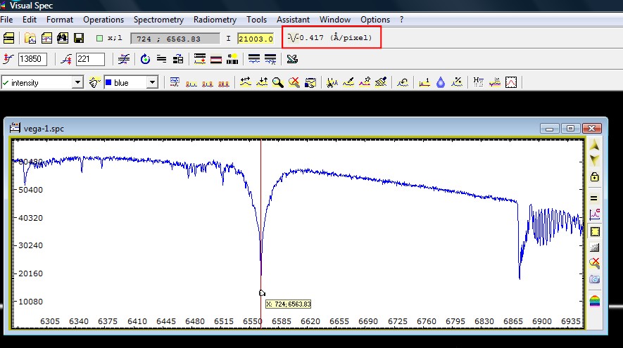
After the processing, the
profile is displayed, the axis is graduated and the sampling factor is
updated in the top toolbar.
I use this
basic calibration extraction during my observing session. I usually
process the first raw image of an object. As soon as the image is
recorded, I open Visual Spec and perform the extraction. As I know the
sampling factor of my instrument, I use the 1 line calibration, just
indicating the H-alpha line position.
|
Spectrum profile basic linear calibration
The function
can be found as a new button in the toolbar or in the menu
spectrometry>basic calibration. A profile
shall be displayed.

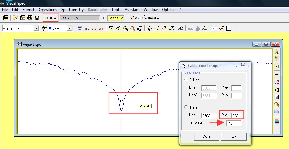
This function
is vary basic. If you know the sampling factor of your instrument, you
can simply assign a wavelength to a pixel value, enter the angström per pixel
sampling value and get your profile calibrated. If you do not know the
sampling factor, you will need to identify two lines and enter the
wavelengths for each line positions in pixel, as described above.
If you turn on the
"next to cursor" XY display, check where is the center of the
H-alpha line. Enter the X coordinate into the box Pixel in front of the 6563
ang value, H-alpha wavelength. Enter the sampling factor, here 0.42
angström per pixel.
If you click in the Pixel
box text field, then click on the profil, the X position will be
automatically updated.
Click ok and the profile
will be calibrated.
Remember, this is not
very accurate calibration, as the center of the line is defined manually. For
better performances, use the 1-line calibration function and select the line
so the barycenter can de determined for better accuracy.
But you can also see the
barycenter of a selected line from here.
Simply select the line
you want to know the barycenter (assuming your profile is not
calibrated). Click the right button of the mouse, a popup-menu will be
displayed. Select the label item. The barycenter will be shown under the
line.
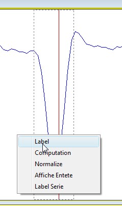 
To erase label, click on
the "refresh" icon in the side toolbar.

|
Default profile window size
As PC screen
are getting larger, the default size of a profile document at opening can be
now modified. Go in the preferences menu. Select the language tab. You
can enter first the width, then the height, in pixels.

|
Image slant and tilt
Load an image.
Click on the
"angle" button. It will compute the slant or the tilt angle.

Slant
If you load a lamp
spectrum, with vertical line, you can compute the slant angle by dragging the
selection (right click of the mouse) around a calibration line. Make
sure the rectangle is higher than its width. This will be the criteria
used by Vspec to define if it has to compute a slant or a tilt angle.

The result is displayed
in the infos window and the slant of the image is corrected.
Tilt
If you load an image of
an object spectrum, then drag along the spectrum, with a rectangle wider than
its heigth. The tilt angle will be computed and the spectrum will be tilted
by this angle.

Note: there is no
possibility in Visual Spec to save images. Those image processing functions
are only for a rapid evaluation of the spectra obtained, on a single
image. And as the correction can quickly be re-applied, this not
critical for this purpose.
For the true image
processings and profile extraction and calibration of an image sequence, see
the ISIS freeware, from Christian Buil.
|
Image rotation
Load an image.
Click on the
"rotation" button.

It will open a new dialog
box.
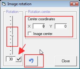
Enter the center of the
rotation in X, Y coordinates. If you want to rotate around the center of the
image, then click on the checkbox Image center. If you want to use the cursor
to define the rotation center, click in one of the text field X or Y, then
click in the image to get the cursor position loaded.
Enter the angle of
rotation in the text field below the slider. To apply it, clcik on the
checkmark icon, pointed by the red arrow.
To come back to the
original image, click on the "undo" blue arrow icon.
You can enter negative
value, and decimal value.
If you prefer you can use
the slider. Click on its small cursor and slide it. The image
rotation will happen upon releasing. Each time you click again on the slider
cursor, the image will re-start from the original one. It is not good to
perform multiple rotation on one image. The quality will be degraded.
The rotation process will
make black areas appear on the side of the image. This can disturb the
good functionning of function like automatic tilt correction. Better to
put then a 0 tilt value and check the tilt angle box in Basic raw profile and
Basic calibrated profile.
In general, applying a
rotation is not appropriate. It will degrade the resolution. It is
recommanded to align at your best the spectrum at the acquisition and use the
tilt function to fix the residual misalignement.
|
Reading bmp files
This is work in progress
function, but it shall be able to read bmp files as image.
In open image menu, in
the dialog box, you can select fits, pic or bmp now as image format
|
Reading dat files
At opening of a .dat
file, check the linearity of the wavelength values. if the mean standard
deviation compare to a linear graduation is greater than 10%, Visual Spec
proposes to resample it. In version 3.9.7 this feature is again removed...
the criteria to decide if non linear is too difficult to adjust and the
message is creating bugs. So, disabled again
|
Export png, jpg, bmp files
You can now export the
content of a profile window as png or jpg or bmp image. It will
keep axes graduation and all annotations.
|
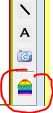
Add annotations on profile
This is again some work
in progress... on the side of the profile window, two new buttons can be
found. One to add a line and one to add a text.

Click on the line
button. Move the cursor where you want the line to start. Keep the
mouse left button pressed and move to the end of the line. Release. If
you want to modify the line, click on it and move one the 2 small dark dot.
If you want to erase, click and press suppress buttton. If you want to add
another line, click again on the line toolbar button.
Click on the A text
button. Move the cursor where you want to put text. Replace the default
text by yours. To select an annotation, click in it. Keep the left
button pressed and move the text to another place. If you click on the small
black dot you can resize the text. If you click with the right mouse button
in a text selected you can change the text position (left, right or center)
and change the police and color. If you want to erase the text, select it by
clicking in it and press the suppress button.

|
Edit utilities files
Visual spec is using some
text file as utilities like the intru_text.txt file which is used to record
all your instrument names or the observation site. You can also have
direct access to the pgm (scripting) files or gnuplot templates etc...
In the assistant menu (a
profile shall be opened) go to the edit menu and pick the file you want to
edit. It will search and open notepad.exe to open the file.

As a result the selected
file will be opened. You can edit the changes and save it. In the
list_instru.txt case, add a new instrument and it will be shown in the drop
down list of instrument when exporting as fit for BeSS (ctrl W)

|
Automatic telluric lines suppression
This is a test. This
function iterates (slowly) on the region 6540nm - 6552nm to eliminates the
telluric lines. If the profile is perfectly calibrated (aligned with telluric
lines to eliminate) this gives some pretty good result. But not all the lines
can be corrected, some overshoot can be seen. This can be
improved in the future.
|
|
V4.0.0
|
Equivalent Witdh
3 new way to compute Equivalent Width are now available in the menu
Spectrometry
- EW lin : from the limit of the
selection, compute the average of the 20 pixels before the beginning of the
selection and the average of 20 pixels after the end of the
selection. Defines the continuum as a line defined by the two above
computed averages. Which lineraized the continuum below the line, which may
have a slope.
- EW cst fit: from the limit of the selection, compute the average of
the 20 pixels before the beginning of the selection and the average of 20
pixels after the end of the selection. Compute the avearge of the two
above average and defines the continuum as a constant line.
- EW cst 1: consider the continuum around the selection is
already normalized to 1, no continuum fit
For all EW computation, compute the Signa to noise ratio from the
region defined as continuum for scaling to 1 operation. See in
Preferences menu, tab continuum. Then compute the EW error using the
formula from Chalabaev, A. and Maillard, J.P. (1983)
It shall be noted that these 3 EW command are also available as
console & script commands: leq, leqc and leq1
|
|
V4.0.5
|
Improved BeSS check
In this version the BeSS
validation check function includes now some tests on the profile wavelength
domain and propose different ways to check the validity of the spectrum.
If the range is large,
Balmer lines are diplayed instead of telluric lines.
If it does not include
H-alphe, He lines can be displayed.
This function is
developped to assist the BeSS administrators to check the submitted spectra.
Use it and see if you can become an admin in the future...
|
Verif Atm cal
This function checks the
accuracy of the calibration using 6 telluric lines around H-alpha region. It
displays the shift onthe graph.

In this example above, a
shift of 0.1 angström would be appropriate
|
|
V4.1.2
|
Opened file list
This function opens a new
window with the list of all the opened files under the current session of
Vspec. It is useful if a lot of files are opened and you are looking for a
specific one, without clicking on the profile window bar to get to the
profile name.

You can get quickly into
it hitting the F4 keypad button as a shortcut.

Click on the file name
you are interested in to bring the profile window on top of all the opened
profiles. Click on the small red cross to close this window.
|
Elements line lists
In this version, 3 new
list of lines are selectable from the elements dialog box. Those are kindly
provided by François Teyssier.
- Neb Plan, refer to a
list of lines generally encountered in Planetary nebula spectra
- WR, refers to a list of
lines generally encountered in Worl Rayet stars
- symb, referes to a list
of lines generally encountered in symbiotic stars
To get access to this new
lists, open the Elements, click on the top right dropdown box and scroll to
see them

|
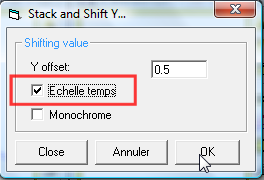
Stack and Y shift, time
When you open the Stack
and Shift Y dialog box, you can the see the options to stack respecting the
scale of time of the list of profiles. If you pick this option, the profiles
displayed in the vspec desk will copy and paste in the current profile
selected. An offset will be added to each profile intensities in regard
to their date and time. The earlier profile will be at the bottom and
the latest at the top with the highest offset added. You can adjust the
"overlap" by playing with the Y offset constant.
If you do not close this
dialog box and you go back to the profile window to click on the display axis
button, the Y-axis will be automatically graduated with the date and not the
intensities. On the X-axis, the doppler display will also be automatically
activated. Make sure the reference wavelength is correctly set. If you
need, you can fine adjust using the Format>Graphics... dialog box.

|
Line analysis
This item brings a new
set of functions to go further in assisting you to analyse your spectrum. It
deserves a specific page on this, so click here to get a deep review of the capabilities.

For planetary nebula this
assistant will help to compute temperature and electronic densities as long
as you have the right lines on your spectrum. It will guide to go directly to
the line of interest and get a measure of them.
For symbiotic, the tool
will only help you to go easely to spectral lines of interest to register
their Equivalent Width. This will allow you to perform time analysis by
collecting spectra at different date and time.
This assistant assumes
the spectra are properly calibrated.
|
|
V4.1.3
|
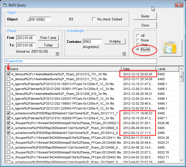
BeSS query
This is an addition to
the BeSS query dialog box. Once the files list if retrieved, we have a
new option list to open only the spectra by month or by year. To open the
selected files, as previously, click on the button with the big icone.
|
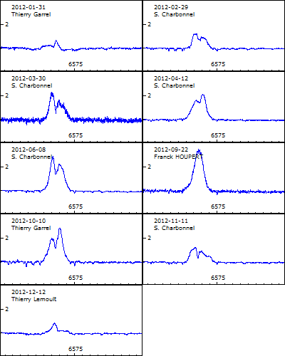
Film composer
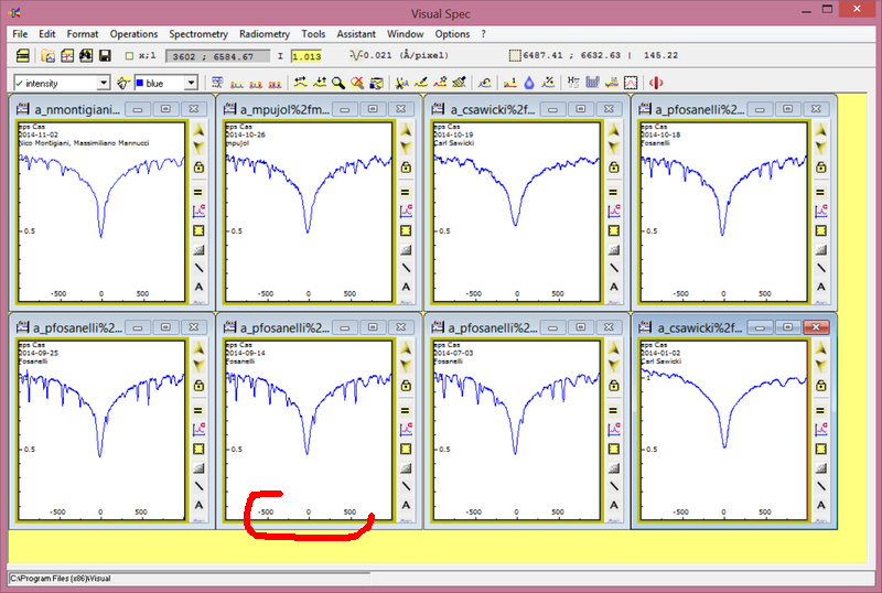
This function generates a
png image made of the thumbnails of the profiles opened in the desktop of
Vspec. You fisrt need to have a set of profiles opened and properly
formatted. Use the window>tile function and the tool>comparison
function to format all the profiles with the same scale and proper axis and
informations displayed.

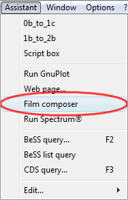
To access to the function
click on the menu Assistant, item film composer.
The function will
re-displayed the profiles according to the settings in the film composer
dialog box from last session.

Change the width or
height of the thumbnail by entering values in the corresponding fields. You
can also change the number of thumbnails per line. Click on generate to
have the new values taken into account. You can also choose to have the
thumbnails ordered by ascending of descending dates.
When you are satisfied,
click on Export button. You can select the directory and the name. By
default, a new directory named "composer" is created in the root
directory of Vspec.exe
All individual thumbnails
are stored by default in this "composer" directory, as bmp file.
From time to time it can be good to erase the accumulated files.

As a result, you will
have the following .png file
Another way to generate
thumbnails is to use the web page generator function. It creates a full
web page with graphics created by gnuplot.
|
|
V4.1.4
|
Directory favoris
In the dialog box to open
profiles, few icons have been added
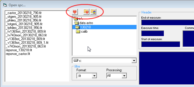
- the change of the
working directory 
- direct access to the
working directory 
- the move to the
directory of the Vspec.exe application 
|
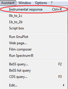
Instrumental Response assistant
This new assistant is
aimed to help in the sequence of operations to compute an instrumental
response from a reference star. This is not to correct objects of the
instrumental response but here to generate it.
You first need to load
the acquired spectrum of the reference star from which you have an
"ideal" profile, and a A-type or B-Type spectral class.
You access this assistant
in the menu "Assistant" when the reference profile is opened.
A new dialog box will
open and the name of the profile which will be used to generate the
instrumentale response. It is recommended to have only this spectrum opened
in the Visual Spec desktop.
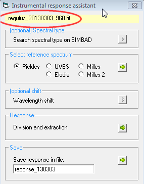
In this assistant the
frame with grey arrow are optional, the one with the green arrow are mandatory.
If you need to know the
spectral type of your reference star, you have a quick access to the CDS
site, with a direct access to the standard CDS query.

The first mandatory step
to generate the instrumental response is the next step.
You fisrt need to have on
your disk the "already corrected profile" for your reference star.
Vspec offers the Pickles database by default. You will pick the right
"ideal" profile which matches the best the spectral type of your
reference star. For Vega, an A0V.
Christian Buil offers an
additionel set of reference spectra with his ISIS software. You can directly installed the data
base where you want. If you install it as isis_database in the vspec.exe
directory, then Vspec detects it and propose 4 news options in the select
reference spectrum frame. If the directory is not present, then the
names will disabled.

To select the
"ideal" spectrum select the database and click on the green arrow

Select the file from the
list proposed. In this example, we have taken Regulus as the reference
star during the observing session. It is in the UVES database.

Click on open when the
uves_regulus.dat file is selected. The profil will be added to the
profile window as a new profile. As you can see below the UVES profile in
purple is slighly shifted from the acquired profile. The optional tool to
shift it and match the acquired profile is provided. This is sometimes
necessary. But you shall also questionned yourself about the accuracy of
your wavelength calibration. (Before extracting the response a good check is
to check telluric lines with the H2O function.)

Here is the final shift

Next step is to now
generate the response.

This will perform the
division and configure Vspec for the continuum extraction

Refer to the standard
operations of this mode. I will show here the most used workflow.
Remove the artefact
produce by the telluric lines
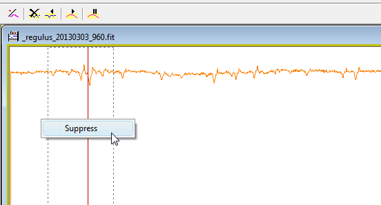
When all are removed, run
the smoothing function

Adjust the fit with the
cursor of the smoothing function.

When fit is ok, click on
the OK button. The orange profile will be moved as the intensity
profile, to be ready for saving.
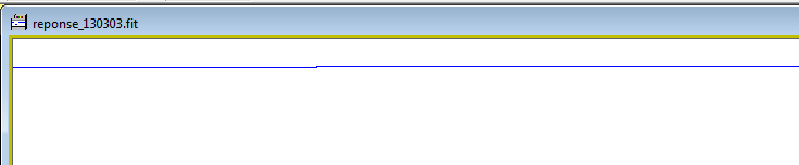
Last step is then to
enter the response file name and click on the green button to save the
file. By default a file name is proposed.

To exit the assistant,
click on the red cross

|
|
V4.2.6
|
Mendeleiev table button
If a profile file is opened, and if the profile is correctly calibrated in wavelength, then you can display the table of element from Mendeleiev. This function is also avaible from the element list window.
.jpg)
A new window will open
and display the table. In this example, the profile is a B-type star (Be
star) and you can expect to see at this temperature spectral lines from
Hydrogene and maybe Helium.
.jpg)
Click on the symbol of
the hydrogene H and Helium He. The spectral which correspond to the element
will be displayed in the coler of the frame clicked. Here, Hydrogene is in
green and Helium is in orange. As expected you can see good matches.
.jpg)
If you want to improve
the superimposition of the Hydrogene line for example, select the serie of
the Hydrogene. You can try using the mouse to click on one of the green line
or go in the serie dropdown list and select it. Then go on the side of the
profile window and click on the Up arrow to increase the scale of the line. The
match with Balmer lines is even more obvious.
.jpg)
|
Adding quick labels
The popup context menu can be displayed by clicking the right mouse button when the cursor is over the image section of a profile window. Select the serie you want to add the date in the graph.
.jpg)
Click on the popup menu and select Label date. The date will be added with the same color than the serie.
.jpg)
As this is a text object, you can select and drag it where you want. You have a similar quick label item in the popup menu to add the name of the object: label name
You can export your image in png format with the save as and select png in the format, or just click on the camera icon on the right side of the profile window.
|
Copy/Paste contextual
To copy and paste a serie from a profile window onto another one you can use the toolbar button or now just use the shortcut in the popup contextual menu. Right click in the image section of the profile and select the copy item.

Select another profile window, rigth click in the image section and select the paste item.

|
Renaming list as sequence
It can interesting to create a sequence like i-1, i-2... i-n from a list of spectra for a same object but at different date of observations. The sequence name i-n can for example be used in ISIS to generate an animation or a 2D image spectrogram interpolated.
Fiirst load all the profile in fits format (can be Vo table from BeSS database too). Make sure date and time are correctly filled. Go in the Assistant menu and select Rename list
.jpg)
A new dialog will be displayed. It will show the list of the file and will prompt you to enter the generic name. You do not need to add "-" at the end of the generic name, Vspec will added for you. Then click on OK.
.jpg)
The files will be duplicated under the new name i-1, i-2, ... and will be stored in your default working directory.
.jpg)
|
Comparison tool with new doppler format
To compare spepctra, it is important to display the profiles with the same format. The powerful tool "comparison" is designed for this. First display the set of profiles you want to compare. Then go in the tool menu and select comparison...
The format proposed by default are Normalization (scaling...) using the wavelength range defined in your preferences settings. Adjust to maximum will detect the maximum intensity across all profiles and pick this value as the maximum Y scale for all profiles.
X common setting will detect the common wavelength range across all the spectra to display all of them at the same X-axis scale.
Display axis will force the display of the axis for all spectra.
Not set by default are the Axe X Doppler, to force the X axis display in doppler scale, the reference wavelength is the one in the graphics options, and the 1000km/s check will force all the Xaxis to be scale from -1000km/s to +1000km/s.
%20(400x258).jpg)
In addition on the right side, you can decide wich labels to add on each profile: date and time, only date, observer name, object name.
It can be useful to refine some axis adjustments before going to the film composer. Go in the graphic settings (double click in the image section, or shortcut Ctrl+G, or menu Edit item graphic, or the two icons in the toolbar with two small arrows). in the Xaxis tab you can check the lambda value which is the reference value to compute doppler shift.
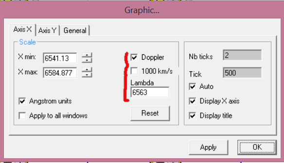
On the Y axis tab, you can see a box called "force". This will preset the ticks and major ticks set to have 0.2 between each tick and no ticks label on major tick.

never forget to click on Apply button. ok button will simply keep the current state and close the box.
|
|
V4.4.0
|
Scaling on all series
When several spectra are displayed in the same window for comparison it is important they are all scaled relatively to the mean on a similar wavelength domain. There is the scaling command which is working on serie by serie base and now here the scaling on all serie button or contextual menu to scale all the displayed serie on a common region of the continuum which can be defined in the preferences or on a specific zone selected if the selection is active (gray rectangle)
The button  is accessible in the toolbar. is accessible in the toolbar.
You can access to the function if you right click in a spectrum window.

Here is an exemple with 2 spectra (in purlple and green) pasted on the original spectrum in blue. A rectangle has been drawn around the area where the scaling shall be based. Reminder: scaling mean all spectrum intensity are divided by the mean of the intensity calculated on a specific contiuum region. This scales all the intentisity in relative to this mean.
|
Local continuum rectification
This fonction divides the zone selected by the local continuum defined as a line between the limits of the zone. This function is of interest to compare locally lines between spectra from different origin which may have continuum imperfections.
Select the zone of the spectrum you want to locally rectify (aka normalize). Then right click on the mouse inside the window to display the popup menu. Select Rectify Locally.
 |
 |
| Before local rectification |
After local rectification on the 2 profiles with scaling |
|
One, two, three gaussian fit
Line fit with one gaussian can be unaccurate when multiple peak are present or when lines are blended. Vspec now has possible fitting with one, or two or three gaussian. It is quite sensitive to the limit of the selection and can take up to one minute to find a good fit. This option is also available in the line analysis tool for nebula or symbotic low res spectrum analysis.
Select the line you want to fit. Go in the menu Spectrometry and pick the number of gaussian fit you want.
 |
 |
 |
| one gaussian fit |
Two gaussian fit on a blended line |
Three gaussian fit on h-alpha line
of a Be Star |
|
Wavelets
Wavelet processing is well known in image processing. This is the 1D version to denoise spectrum by adjusting wavelet parameters.
*** warning*** this processing is NOT to be used on data before scientific database submission.
Open a profile. Go in the menu operations>wavelets. A new window is opened

The profil is decomposed into 8 consecutive layers. Each of the layer is shown in the small graph on the top left zone. if you want to remove noisy layers, unclick the checkbox and press Recon. The result is displayed in the graph at the bottom left.

You can also play with thresholds on the layer before your recombine them. Use the check box on the right in the filter section and enter manually threshold.
Then click on export to display the denoised profile in orange as a new serie named intensity.ondxxx with x the layer order starting at 0

See below overlayed on the original noisy profile in blue and window expanded.
|
EW time series
Up to now, it was possible to generate Equivalent Width time serie using the script box and a pgm. The display was not adressed. now you can display the curve using gnuplot with either Julian day or normal date format in abscisse. The input file is still a dat file with can also be read by any external software.
Open all the files which will be used to compute the time series. Generate the EW time serie using the script box and a program like
Load $1
leq 6540 6585 <- compute the Equivalent witdth between wavelength 6540 ang and 6585 angstrom

The results are displayed in the infos windows and a file named leq_[objectname]_[date].dat and leq_[objectname]_[date].dat are created and stored in the vspec.exe directory.

Go in the tools menu> gnuplot EW or gnuplot EW julian date
 |
 |
| With date in standard format jj/mm/yyyy |
With date in julian day |
The gnuplot graphic is displayed and the png files are stored in vspec directory.
|
Batch menu
This new menu is proposing operations on a serie of spectra
File list processing - this new tool will allow you to compute
- Equivalent width... similar to the script box with pgm function but a more direct access providing user enters the range over which the EW will be computed. This function does not display the continuum orange curve so is much faster and the graphic display the error bar.
- Maximum... detect the maximum over the range selected for each opened spectra and store the results in file named max_[objecname]_[date].dat - Store the maximum intensity along with the date. Gnuplot display at the end.
- Chrono Spectrogram... an image of all the spectra in intensity as grey values, interpolated or not and the capability to generate from there a 3D print surface compatible with openSCAD to create an STL file
Average profil - this creates the average profil from all the spectra opened. Makes sure your spectra are not displayed in km/s before generating the mean profile.
|
BeSS check with automatic copy/paste
To increase the efficiency of pre validation of spectrum before submission to BeSS, for spectral resolution above 4000, an automatic copy/paste of the last 2 beSS spectra and a scaling of the pasted profile are now performed.

if you do not want to perfom the automatic scaling you can disable this in the preferences menu, tab continuum.

|
File processing batch
This a powerful new tool window.
To fill the list of profiles, look at the left buttons

Button Clear List will clear the list
Button VSpec files will fill the list with the profiles which are currently opened in VSpec
Button BeSS query will trig the BeSS query window. Once your query is done, click on export list to fill the file processing tool list. It has to be noted that if you start by performing a BeSS query then clicking on exort list will automatically call the file processing tool

Once you have you list of profiles set, pick the task you want to perform from the button on the top right

|
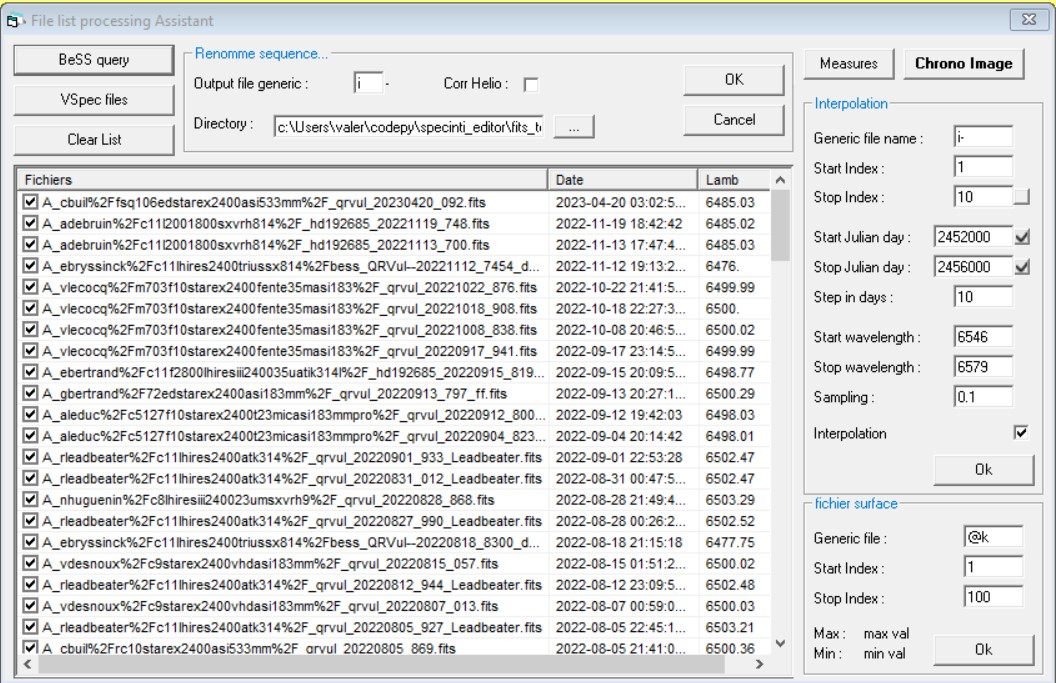
Chrono spectrogram
You access to the configuration by clicking on the Chrono Image button. By default this panel is displayed.
The first action is to generate the profiles as a sequence of files numbered. Refer to the middle up zone.

Enter the generic file name, here by default it is "i"
Select the directory where your i-1,i-2... i-n files will be saved by clicking the the 3 dots button - the directory shall pre-exist

***Only if files from BeSS**** you can activate the Heliocentric speed correction

Once all is set, click on OK to generate a renamed sequential files copy in the directory you set.
Now look at the left "interpolation" zone
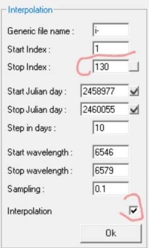
- Generic file name : you find here the name of your previous renamed sequential file list - this field can be used if you have generated your own sequence with another program, but make sure you have select the correct directory in the rename section and adjust the number of file and all configuration values of index. if you click on the small cross next to julian days it will update the field from the start and stop indexed file.
- Start, Stop Index: index of the first,last file to consider for the chrono spectrogram - automatically updated after the rename action
- Start, Stop Julian day : a temporal way to sub-select files for the chrono spectrogram
- Step in days: select the step of the lines in the 2D chrono spectrogram
- Start, Stop wavelength : select only a wavelength range of interest - the more data points you have the longer will be the 2D image generation
- Sampling : resample all the profiles at the sampling value in angström - this also limits the number of data points
- Interpolation: check box to activate or not the interpolation at the step in days
When all is set you click on Ok and let the program runs...
Once done, you will see a new image window like this, you can resize the window.
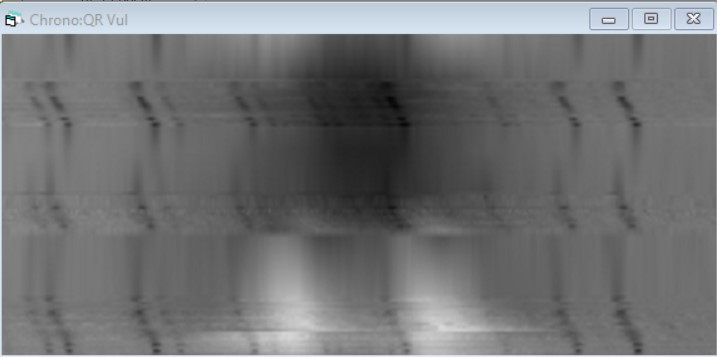
This image is the result of QR Vul BeSS spectra from the last 3 years. As it is corrected from the heliographic speed the telluric dark lines changed position. But we can see at the bottom the 2 peaks in emission of the H-alpha, then is absorption and restating again an emission phase. The top of the diagram are the most recent dates.
If you move the mouse over the image you will see a colored label. When yellow the intensity line is an interpolated one.

When blue, then it is a true profile of your time serie - the image below is with a smaller value for interpolation from 10 days above to 2 days below
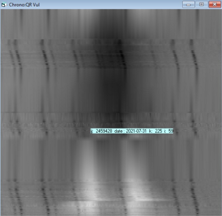
You can play with the parameters to select a temporal subset or a wavelength range or play with the step in days for interpolation.
If you want to print in 3D then look at the next section...
|
3D print of serie of spectra
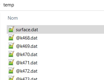
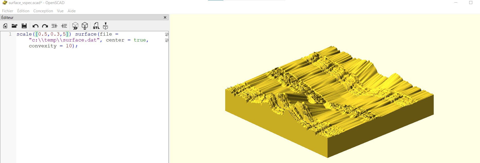
Once you have generate your 2D chrono spectrogram, then you can generate a surface file. The format is compliant with the 3D stl program OPENSCAD, a freeware for building 3D volume and STL file generation.

It is prepopulated after you generate the 2D chronogram. You will see the surface.dat file in the directory
Then open the openSCAD program and enter the small code
scale([0.5,0.3,5]) surface(file = "c:\\temp\\surface.dat", center = true, convexity = 10);
You have to specify the directory where the surface.dat file is and adjust the parameters in the scale command. Then click on the small button with the double >> to generate the 3D volume in yellow on the right.

The volume once you click on >> button
You mave have to play with the mouse to zoom in-out and orientate the volume. Once you are happy with the scale parameters, click on the button with STL to generate your stl file to enter in your 3D Printer and enjoy !
This is a 3D print of full time serie of BeSS QRVul printed in 2021

|
Measures on time serie
If you want to compute a curve of a measure on the file list, click on the measure button
The left panel will change

The most interesting measure is the Equivalent width.
Enter the wavelength start and stop where the EW shall be computed. Then click on the Ok button in the Equivalent Width zone. The computation will start and you will see it at the end as a gnuplot. Every profile measure and in the blue window. The gnuplot file is saved in your current working directory under the name leqjj QR Vul 05-06-2023.png and the dat file in ASCII you can use in another plotting software.

The max measure is more tricky as it generates a curve with the max value of the wavelength domain you specify. This is only relevant for pure emission line profiles.
|
|
|
|
.jpg)
.jpg)


