by Christian Buil
The Solar Explorer - October 25, 2023
by Christian Buil
The Solar Explorer - October 25, 2023
Processing

This section describes how to extract the Sun images saved in SER files with Sol’Ex, as well as how to process these images. The common thread is an acquisition made on September 5, 2021 at the H-alpha line wavelength by coupling Sol'Ex to a 65 mm diameter refractor and 420 mm in focal length (TS model), typical of the equipment used with Sol 'Ex. The camera is an ASI178MM operating in 2x2 binning. You can download this observation as a SER file named 12_08_34.ser, along with supporting files produced by the SharpCap software at the time of capture. To do this, unzip the ZIP file available on this link, 12_08_34,, in the directory of your choice (for example c:/capture/).
I will discuss two software that can run from the Windows environment. First, the INTI software, which specializes in decoding SER files and producing ready-to-use images of the Sun. Then the i-Spec software, also capable of extracting images of the Sun from your "scans", but of more complex use, and above all specialized in the processing of these images.

Part 1: INTI
INTI is a project initiated and developed in Python by Valérie Desnoux with the help of a handful of collaborators. Great care has been taken so that you can use this software on your computer without having Python installed, or even having any knowledge of this language. INTI presents itself as an ordinary Windows application in form.
INTI is very easy to install. For the procedure and to download the application, go to the site: http://valerie.desnoux.free.fr/inti/
Let's see immediately how to use INIT by exploiting the 12_08_34.ser file. Start INTI, click on the Open button then select the SER file:
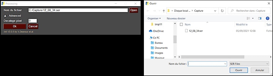
Secondly, you click on the Ok button, and INTI carries out number of calculations in a fully automatic way: reading of the SER file, correction of the transversalium, evaluation of geometric distortions, synthesis of Quick-look images to give you a quick idea of the result, save the images resulting from the processing in PNG and FITS format in the directory from which you loaded the SER file.
Most of the work concerns geometric corrections. They are two types, and you have to know how to recognize them. The first correction concerns the difference scale along the horizontal axis (SX) and along the vertical axis (SY), which can make the images look like a rugby ball:
In this example, the SY / SX ratio is less than 1. This means that the frame rate against the disk scan speed is too high. We say the image is oversampled. A SY / SX factor between 0.75 (as in this example) and 1 is quite acceptable. By aiming for the value SY / SX = 1 we reduce the size of the SER files. The situation to be absolutely avoided is that of a scale factor less than unity:

This result indicates that the frame rate is too low. It is catastrophic because it forces the software to extrapolate the image to end up with a circular disk, that is, artificial information is produced. The result is a marked loss of resolution in the final image. Be careful when observing!

The second correction is tilting correction, if needed. The tilt angle in this example is 5 °, a high value that can be seen clearly on the image itself. In addition, there is a lack of scale here. You can try reducing the angle to 1 ° or less, it is doable, and always better, especially if the disc is sticking out of the sensor frame, to reduce truncation in the edges.
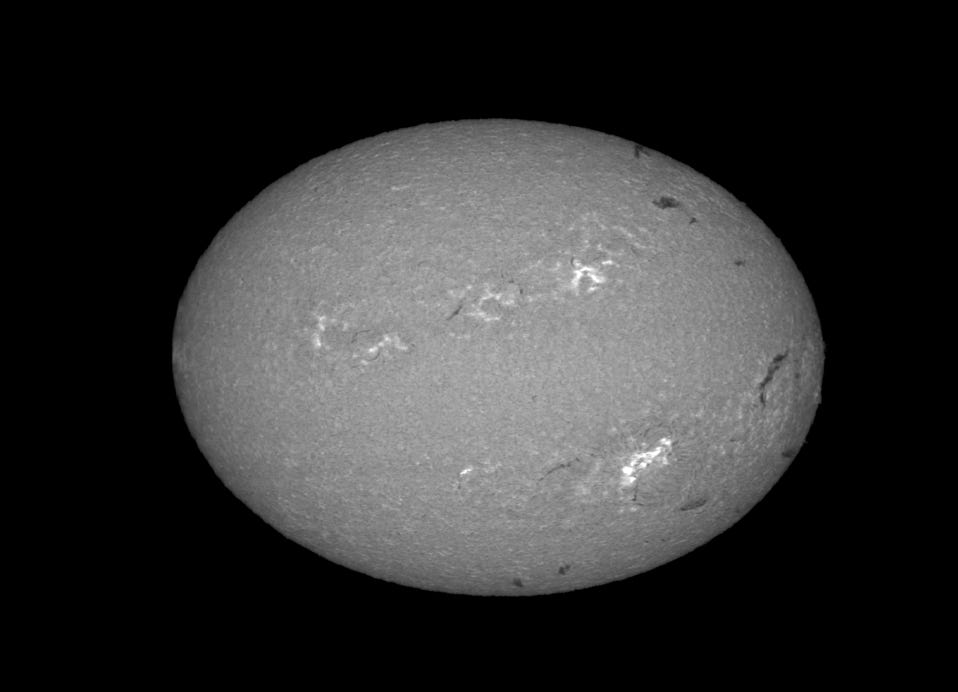
INTI is very good at correcting these distortions automatically. Here is the final result generated by this application:

At the end of the calculation, INTI displays a certain number of images on the screen which allow the result to be evaluated. They remain present for one minute, but you can also exit this mode by pressing the “Return” key. Among other things, you have at your disposal a visualization of the protuberances:

You will find these images in the graphic PNG format in the working directory, but also the versions in the FITS format, the standard in astronomy:

The most important FITS file for us, because it is the purest actually processed image, is the one whose name ends with "xxx_recon.fits". Here it is the file "_12_08_34_recon.fits". Another important file to watch out for is the one whose name ends with "xxx_raw.fits". This is a so-called "raw" image file that allows you to judge the appearance of the image before correcting geometric distortions, which allows you to judge the situation at the time of acquisition.
INTI also saves a text file “_log.txt” which contains the results of calculation, and in particular the factor SY / SX evaluated. In our example SY / SX = 0.98, which is fine:

Another valuable information concerns the coordinates of the center of the disc (XC, YC) and its radius in pixels. These data will be very useful for the future.
INTI performs the calculations quickly and automatically. It is an ideal companion even as you observe the Sun, to analyze the situation and make it attractive. We are certainly not in real time, but the level of interactivity is already correct.
Part 2: i-Spec
Part 2.1: Configuration
I-Spec is an application written by the author (derived from a more complete software, ISIS), particularly optimized for the exploitation of Sol'Ex (and also Star'Ex, with some possibilities in terms of exploitation of spectra ).
Remember at this stage that i-Spec allows you to decode SER files, perform arithmetic operations on images, perform geometric operations of any type, etc.
You can download i-Spect from this link: i-Spec.zip. All you have to do is unzip the ZIP file in the directory of your choice and launch i-Spec.exe (you can also copy the icon to the desktop).

In particular, you must define the working directory, and choose the .FITS extension for FITS files. These settings, and many more, will be left as they are when you relaunch i-Spec. You can also choose here an English language interface (re-run the application).
Part 2.2: Quick-Scan
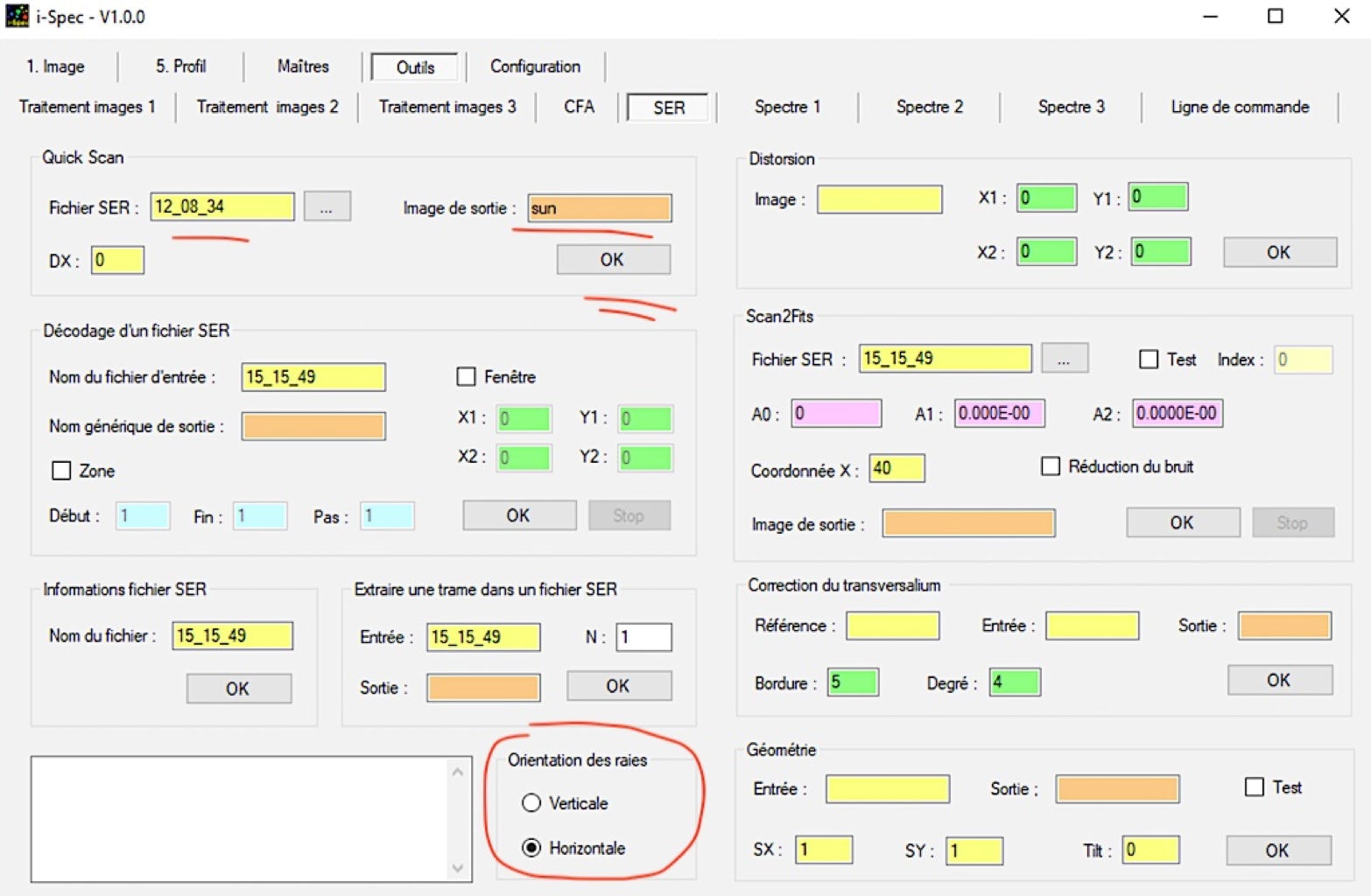
Click on the "Tools" tab, then the "SER" tab. You are then in your main working environment. The first and very important thing to do is to tell i-Spec that we are working on SERs in which the lines are recorded in a horizontal orientation (this setting will be kept, until you change it) . Then, as shown in the following screenshot, in the Quick-Scan area, enter the name of the SER file to be processed (you can use the "..." button to open a file explorer). Also indicate the name of the resulting FITS file, the extracted disc image - here we entered "sun", but you are free. Then a click on "Ok":
The calculation is fast (faster even than with INTI because here i-Spec does not make any geometric correction and the processing technique is simplified for the benefit of speed). The image file is as it was acquired (equivalent to the RAW file under INTI) and saved in the working directory. To see the result, click on the "Image" tab. We want to visualize the "sun.fits" image created in the previous step. You enter the name "sun" (no extension in the file name), then click "Show" (or Return, when the cursor is in the file name entry area). You can also find the image to display using a browser (button in the right part of the window):

The image of the Sun is displayed in its capture format. Get used to manipulating the sliders at the bottom of the image to adjust the brightness and contrast (high and low thresholds). If you are satisfied with the visualization, you can save it as a PNG file (infographic) by clicking on the "Save" button:

Remember to select the PNG button, otherwise a FITS image is saved. The result is in the working directory. Given the speed of operations in Quick-Can mode, note that i-Spec can also be used at the time of acquisitions.
Part 2.3: How to extract one frame from SER file
For some operations or controls, it may be useful to extract one or more images of the spectrum from the SER file (this file may contain hundreds of frames, or images of the spectra acquired at high speed).
Still from the "SER" tab, you have two solutions.
Use the "Extract frame to SER file" tool. The usage is obvious: you give the name of the "SER" file, then the row of the frame:

In the example, it is the frame of rank 982 which is extracted, which corresponds approximately to the central image our SER file which contains 1964 frames (you can obtain this information using the “SER file information” tool) . We choose to call this snippet of the SER file with the name "frame" (you have all the choices. This is a new FITS file saved in the working directory.
The other way is to use the "Decode SER File" tool. You have several choices, for example with the possibility of extracting all the frames from a SER file as separate FITS files, or as here define a zone (limited to frame 982 in the example). This time the name "frame" is a so-called generic name, which means that i-Spec adds an index number after the name. In this case, the software will produce the image file trame1.fits. If you set the extraction zone to 621 for the start and 623 for the end, i-Spec produces the files trame1.fits, trame2.fits, trame3.fits. This makes it possible to carry out a very fine analysis of the analyzed scan, image by image.
Of course, we use the "Image" tab to display the result:

The very threadlike portion of the spectrum (the cropping area under SharpCap) corresponding to frame 621 and is displayed with a horizontal dispersion axis (the "norm" in spectrography).
Part 2.4: Spectral distorsion function
We know that the shape of the lines has a curvature. This curvature can be modeled by a polynomial of degree 2 in i-Spec. We will calculate the coefficients of this polynomial.
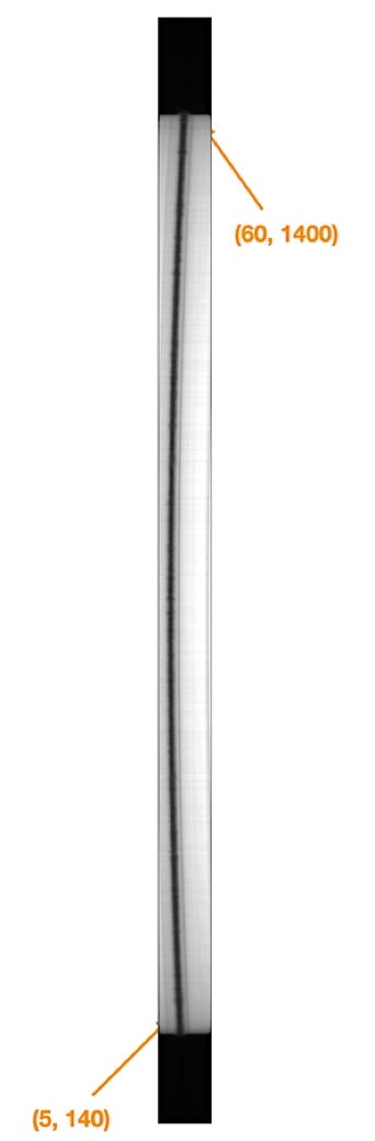
With the help of the cursor, you note the coordinates (X, Y) of the opposite corners of a rectangle which surround the line, see the example opposite. There is no need to be precise, the main thing is to frame the line.
You enter these values in the "Distortion" tool, specifying the name of the image for which the calculation is applied:

-Spec returns the value of the coefficients of the polynomial after pressing "Ok":

During these operations, two control images which have been saved in the working directory. The image "check1.fits" shows the points in the heart of the line that were used to calculate the parameters of the distortion of the H-alpha line. The image "check2.fits" shows the straightened shape of the line. Let's display this last image from the "Visualization" tab:

The "Scan2Fits" tool generates the image of the disc with the parameters calculated previously (note that some fields are already pre-filled). The X coordinate is that of the center of the H-alpha line (noted on the image "check2.fits", see left). You then do OK, this time with a significantly longer computation time. Here we decide to call the disk image "disk1":

You can of course examine the "disk1" image from the "Image" tab. If you notice any horizontal lines, this is the transversalium caused by flaws in the slot, you can try to erase them with the "Transversalium Correction" tool. You duplicate the name of the image to be processed in the "Reference" and "Input" fields. You give a name to the image to be processed, here "disk2". The “Degré” parameter sets the detection factor of the traversalium. The value is typically between 4 and 8 - experiment. The border parameter makes it possible to eliminate edge effects (artefacts) at the north and south poles after treatment of the transversalium. Here again, experiment and see how the settings work. Let's adopt for example:

The last operation to be carried out concerns the geometric corrections. Unlike what INTI does, it is manual, but it also offers more control. We use the “Geometry” tool. For example, do:
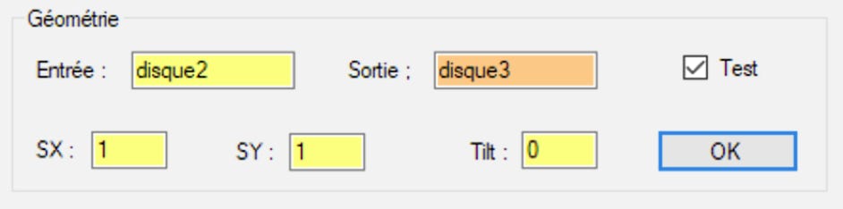
We decide here not to carry out the correction of the scale factor since SY / SX = 1 nor of the tilt, since the angle (in degrees) is zero. Notice that the “Test” box has been checked. When we display the image "disk3" this is what we see:

By being attentive you will see a dotted circle which surrounds the disc of the Sun. At the poles, this circle does not exactly follow the contour of the disc. This is a sign of a slight defect in the SY / SX scale. We now apply the value found by INTI, or SY / SX = 0.98 (but reversed because a correction is made):

Now the solar disk appears perfectly round (test several values of SX, SY and Tilt, sometimes it will be necessary to act by iteration). Take advantage of the situation to note the coordinates of the center of the disc and its radius in the result window on the right. Rounded to the nearest pixel, we have here XC = 1016, YC = 769, R = 646. Then relaunch the "Geometry" tool, but unchecking the "Test" option, which will eliminate the circle.
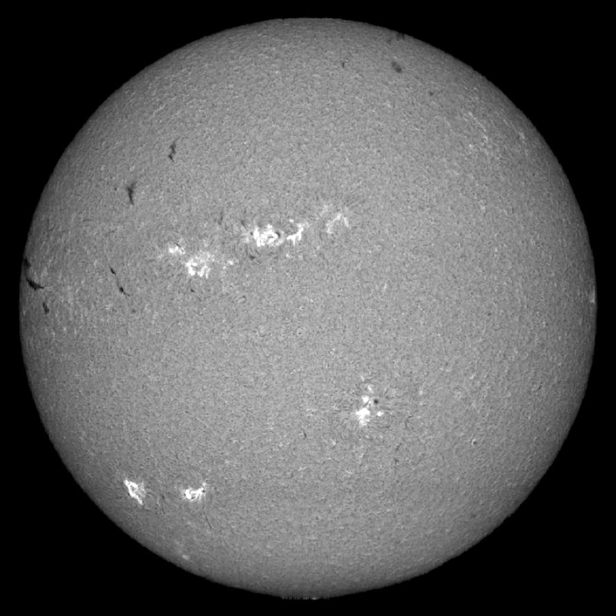
From the "Visualization" tab, save the processed image in a FITS file with the final name. You can also save a file in BMP format, which exactly reproduces the current visualization on the screen. Here is our final image:

From there, there are plenty of possibilities. For example you can use the many functions accessible from the command line of i-Spec (the description of all these commands is beyond the scope of this introduction).
From the "Tools" tab, open the "Command line" tab. In the box at the top of the window type the command:
disk1 disk3 protu 1016 769 646
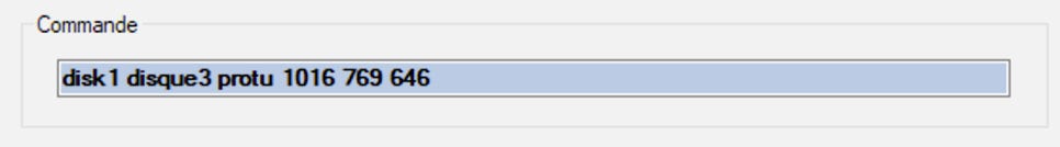
Then type "return". You have surely understood that the numerical parameters are the coordinates of the center of the disc and its radius. If you have any doubts about the syntax of a command, simply type its name and then "Return". You can recall old orders with the up and down arrows, you can modify them, relaunch them by pressing "Return" wherever you are in the edited line ... The i-Spec command line is a "production tool" " very effective.
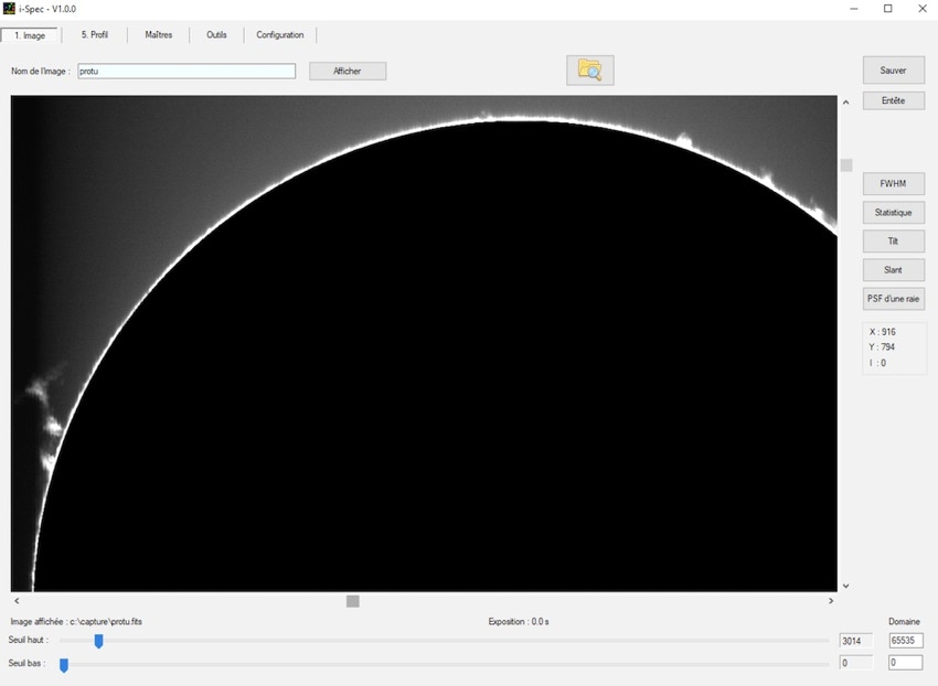
i-Spec generates from the command "disk1" the image of a hidden disk, which highlights the protubernces:
Whether you use INTI or i-Spec you can perfectly choose the length from which you synthesize the disc from a single "scan". Below is the image in the heart of the H-alpha line (X = 18), in the wing of the line (X = 21, i.e. an offset of 3 pixels, which represents 0.37 A or 17 km / s - see part 4 of the “Construction” section), in the continuum (X = 40, we only see the photosphere and the spots) and finally an image of the solar rotation by exploiting the information of the red wings and blue of the H-alpha line:

X=18
X=21

X=40 -> photosphere
Chanel R -> X=16 - Canal V -> (16+ 20) / 2 - Canal B -> X= 20
It is with these simple techniques that you can probe the depths of the Sun's atmosphere, measure velocity fields, reveal the Sun's rotation, etc. The amount of information contained in a single scan of the record with an instrument like Sol'Ex is considerable. It's up to you to discover and use it!

You can even perform a sunset "scan" as it crosses the horizon.
Partie 3 : Utilities
Part 3.1 : CheckSun
CheckSun is a powerful online utility written by Matthieu Le Lain to interactively compare your images of the Sun with those of professionals in near real time (satellites, etc.) or even to check their orientations. Available at: https://checksun.stellartrip.net
A video showing a quick example of use is available here: https://www.youtube.com/watch?v=EplKc9XYPCg

The repository of sources is available at this address: https://gitlab.com/matthieulel/checksun
Part 3.2 : Some Web adress
BASS 2000 : https://bass2000.obspm.fr/present_fr.html
NSO : https://nso.edu
Current Solar Images : https://umbra.nascom.nasa.gov/newsite/images.html
Solar Monitor : https://solarmonitor.org
MLSO (K-corona) : https://www2.hao.ucar.edu/mlso/mlso-home-page
Solar Dynamics Observatory (SDO) : https://sdo.gsfc.nasa.gov
SOHO : https://sohowww.nascom.nasa.gov
STEREO : https://stereo.gsfc.nasa.gov
Big Bear : http://www.bbso.njit.edu/cgi-bin/LatestImages
Helioviewer : https://www.helioviewer.org
USET : http://sidc.oma.be/uset/
Observatory Kanzelhohe (home) : https://www.kso.ac.at/index_en.php
Observatory Kanzelhohe (ephemeris) : https://www.kso.ac.at/beobachtungen/ephemeris_en.php
Copyright (C) 2020-2023 Christian Buil
Web : www.astrosurf.com/buil