|
HF
Propagation tutorial
by
Bob Brown, NM7M, Ph.D. from U.C.Berkeley
Distribution
of ionospheric electrons (III)
In
the previous page, it was pointed out that further progress on
propagation requires knowledge of how ionospheric electrons are
distributed. Of course, that will be different, day and night, as
well as with seasons and sunspot cycles. Again, it would be easy way to
fall back on something in the introduction,
say the night-time ionosphere and continue the discussion from there.
But that would
involve a tremendous leap over distance and logic that's not too
productive. So let's talk/walk our way up to higher altitudes,
starting from where we are now, the D-region.
For
one thing, the D-region involves a lot of familiar ideas and we can
work from there. For
example, below the 90 km level, our atmosphere is pretty well mixed,
about 78% nitgrogen molecules and 21% oxygen molecules, by volume. The remaining 1% is made up of permanent constituents, like
the noble gases as well as hydrogen, methane and oxides of nitrogen.
Of course, every schoolboy knows about the variable
constituents, like water, carbon dioxide, ozone and various bits of
industrial debris, smog, that are found in around heavily populated
regions.
Global
weather systems keep the lower atmosphere all stirred up, in a
mechanical sense, but that is not to say that convection from solar
heating is the only influence of the sun. Indeed, as was discussed earlier, there are electrons and
positive ions in the lower D-region, released by solar EUV and
X-rays. When the sun sets, one might think that all the ionization disappears by
recombination and the region becomes de-ionized and neutral.
 |
 |
|
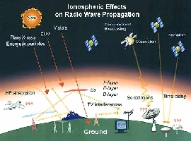
At
left structure of the neutral atmosphere et the
ionosphere. At right closeup on the ionosphere layers
where charged particles (electrons and ions) of
thermal energy are present, which are the result of
ionization of the neutral atmospheric constituents by
electromagnetic and corpuscular radiation. At night
the D-, E-, F1 and F2-layers vanished and are replaced
by the F-layer located higher in altitude. The lower
boundary of the ionosphere coincides with the region where the most
penetrating radiation (generally, cosmic rays) produce
free electron and ion pairs in numbers sufficient to
affect the propagation of radio waves (D-region). The
upper boundary of the ionosphere is directly or
indirectly the result of the interaction of the solar
wind with the earth upper atmosphere. On the
night-side the ionosphere can extend to greater
distances in a tail-like formation, representing the
solar wind shadow. In the tail the extent of the
ionosphere is limited by the condition for ion escape. |
|
Of
course, the ionosphere is always electrically neutral, with the
equal numbers of positive and negative charges, but recombination
lowers their numbers. Still
some ionization does remain, produced by other sources; those
include UV and X-ray photons in starlight, sunlight scattered by the
gas envelope (geocorona) surrounding the earth and even charged
particles, the energetic protons in the galactic cosmic ray beam.
So
it follows that ionospheric absorption would be greatly reduced
after dark but does not go to zero. There is good news in this discussion, however, as some
electrons are taken out of the absorption loop at night by becoming
attached to oxygen molecules. Those negative ions are so massive
that they can't be budged by RF going by and just do not participate
in the absorption process.
And
at night, the number of negative ions of molecular oxygen in the
lower D-region grows to large numbers in going downward from the 85
km level. That is the very reason that those solar proton or PCA events
mentioned previously show much less absorption when the sun
sets. But when the sun comes up, solar photons detach electrons from the negative ions and
absorption goes back to the daytime level again. That does not happen for auroral events and that is another
story, about another region higher in the ionosphere. More on that later.
In
any event, the frequency dependence is still in effect for whatever
absorption occurs, taking a heavy toll on low frequency signals. But that
is still not fatal to propagation, even on the low bands. Thus, everyone
knows about broadcast stations coming in better after dark and those
signals can be heard across very great distances, as many SWLs will
testify. And even with more limited power, 160 meter operators can still
work great DX. But in the last analysis, both SWL and low-band DXers run up
against the same problem, noise. That also has its origins down at low altitudes so we can
deal with that right now, while in the region.
Noise
is described as broad-band radiation from electrical discharges,
either man-made or natural in origin. Whatever the case, being a radio
signal, noise will be propagated like any other signal on the same frequency.
That means, for one thing, that noise signals that are below
the critical frequency of the F-region overhead will be confined to
the lower ionosphere, dissipate down there and not escape to
Infinity. By the same token, noise signals above the critical frequency
are lost and won't bother us very much on the higher HF bands. But the
lower bands do have a problem; so let's talk aboutit.
Noise
of atmospheric origin comes from lightning strikes and will be
seasonal and originate in fairly well-defined areas. Among the
powerful sources of noise are low-latitude regions
of South America, South Africa and Indonesia. But the U.S.A. have
their own noise source too, the southeastern states
during the summer months. So broad-band noise originates from those
regions and is propagated far and wide through regions in darkness.
But once the sun comes up, ionospheric absorption takes over
and the only noise heard is of local origin, static crashes from
nearby lightning strikes.
The
above points are not news to domestic DXers; they are quite familiar
with their own situation and can work within its limits. But those
going on DXpeditions often go into unfamiliar territory and don't
always think about the atmospheric noise problem. So 160 meter operators on DXpeditions have been known to be
greeted by S-9 noise the first time the receiver was turned on. That evokes instant panic and sets in motion efforts to
ameliorate the problem, say trying different antennas and such. Those don't work every time and hindsight often proves the
problem could have been avoided, in large measure, by planning the
DXpedition for a time on the winter side of an equinox, not the
summer side.
Of
course, the other source of noise is quite local, man-made in origin
and coming from various electrical devices. While the global dimensions of atmospheric noise have been
investigated extensively over the last 50 years or so, the same is
true of man-made noise and it can be categorized as to origin and
even given a frequency dependence.
As
for origins, the worst situation is an industrial setting and then
lesser problems are found with residential, rural and remote sites,
in that order. In that
regard, the IONCAP propagation program allows one to select the
receiver siting and then takes that, as well as the bandwidth (in
Hz) of the operating mode, into consideration in calculating the
signal/noise ratio that would be expected for a path.
Of
course, an operating frequency is put in for each calculation,
giving results for noise power similar to the rough sort of
frequency variation shown at left.
It
should be realized that those values for the noise power are
averages throughout a day and subject to considerable variation,
with changes in human activity.
So low-band DXers sitting there in the wee hours of the
morning will not hear the buzz of chain saws or weed-eaters but they
might have to put up with other noise, say sparking heaters in fish
tanks or hash from computers, TVs or various forms of consumer
electronics in nearby homes.
Last
of all, there are extraterrestrial sources of noise too, from the
galaxy, as noted in regard to riometers, and solar noise outbursts.
Galactic radio noise is quite weak and reception requires
very sensitive receivers at sites well-removed from sources of
man-made noise. But solar noise is another thing and it can be quite
strong at times when solar flares are in progress.
As
you'd expect, solar noise can pass through the F-region if its
downward path has an effective vertical frequency that is greater
than the critical frequency of the F-region. Thus, solar noise would
be heard more often at the top of the amateur spectrum, especially
when the sun is at a high angle in the sky. And it can be
quite strong at times, whooshing sounds that rise and fall in
intensity, even capable of overpowering CW and SSB signals on the
higher bands. By way of
illustration, solar noise was discovered by British scientists
during WW-II and was first thought to be a new form of German radar
jamming. OK?
Extraterrestrial
noise sources are getting a bit far afield so we'd better get back
down in the D-region and move on from there, going above 90 km and
seeing how matters start to change.
Now
we have to move up from the D-region, going above 90 km into greater
heights. In doing that, it is necessary to not only talk about the ionosphere but also the
underlying neutral atmosphere.
A
few words about the ionosphere will do for starters since that is
something we've already covered. For example, the collision frequency of electrons with their
neutral surroundings is quite important in discussing ionospheric
absorption. And I mentioned that falls off with increasing altitude.
The same is true of the collisions between the neutral constituents.
So neutral-neutral collision frequency goes from about 6.9x10¹⁰/sec at
sea level to 1.2x10⁴/sec at 90 km, dropping about six orders of
magnitude. The same is true of the number density, going from 2.5x1025 particles per cubic
meter at sea level to 5.9x10¹⁹ particles/m3 at 90 km.
Clearly,
things thin out as we go up and collisions become much more
infrequent. Of course, you suspected all that but now you know some of the numbers.
But you may have not suspected how those changes would affect
DXing on HF, even VHF. So stay tuned as I go a bit further; then I will get
to the "nuts and bolts".
To
go on, I mentioned the atmosphere is lightly ionized and I also
pointed out that recombination was the fate of electrons and
positive ions, especially after dark. But it does go on even in the sunlight and one process
involves recombination of positive molecular ions of oxygen (O++)
with electrons. When
that happens, the neutral molecule (O2) is re-formed but with excess
energy; so it flies apart, into two oxygen atoms (O). But considering how lightly ionized things are in the
ionosphere, that can hardly be considered as a strong source of
oxygen atoms. OK?
But
during the day, the atmosphere is bathed by energetic solar photons;
some, as we know, ionize oxygen molecules and thus can contribute to
the ionosphere. Others dissociate oxygen molecules into two atoms.
But with such a low collision frequency at 90 km, an oxygen
atom can linger around for about a week before finding another
oxygen atom and recombine to form molecular oxygen again.
So
the long and short of it is that by the steady illumination of the
atmosphere by the sun, atomic oxygen can build up to become an
important constituent of the atmosphere above 90 km. One step further
tells us the atomic oxygen ions, O+, will be
created too by all those solar photons going by. So how long will those ions last?
Good question; it depends on which process is considered,
perhaps recombination with an electron to form a neutral atom. It turns out that if recombination were the only possible
fate for O+ ions, they'd linger around a long time too. Something else seems to happen but before getting to that,
let's look a bit deeper into the O+ situation up above 90 km. OK?
The
recombination of O+ with an electron is a radiative process, the
excess energy being given off as a photon while the atom recoils to
conserve momentum. But it is slow , I mean VERY SLOW in the scheme of things.
And that seems to be the case for other similar radiative
processes, like with metallic ions. It just seems to take forever for an electron and metallic
ion to get it together and recombine. But now comes the PUNCH LINE; there are metallic ions in the
upper atmosphere, meteoric debris that has drifted down and been
ionized by solar photons.
|
|
|
Ionospheric
effects on radio waves propagation. Document IRPG. |
And
recombination being a slow process, they linger around a long time. In fact, they can linger around and be caught up in the
occasional weather activity up around 100 km, wind shears. And being tied, as it were, to field lines, wind shear can
compress them into a thin layer. But their electrons are not far away so that makes for a thin
layer of electrons too. So now you guessed it; I'm talking about sporadic E layers up around
100 km or so.
The
electron population, being squeezed into a thin layer, looks sort of
metallic too when it comes to wave propagation so RF is really
reflected by those layers, the sort of thing we talked about in the
introduction, tilted reflecting layers. In the present case, the tilt would be that of the magnetic
field lines that hold the charges. But the tilt is not so important
to DXers; it's the presence of a strong, reflecting layer around 100
km altitude.
Sporadic
E is known to be a nuisance for HF propagation. By its presence, it can RF cut off from long paths via the
F-region up around 300 km and thus disrupt long-haul communications.
And the reflecting properties can be so great as to not only
reflect RF from the top of the HF spectrum, to the annoyance of 28
MHz DXers, but also reflects RF in the VHF portion of the amateur
spectrum, to the joy of the 50 MHz and 144 MHz DXers. I should
add that some contestors love sporadic E as they can
go to higher bands and make many short-haul contacts on bands that
would be quite dead otherwise. All that from the fact that recombination
is so slow for atomic oxygen and metallic ions.
Still
speaking about the importance of atomic oxygen in the atmosphere
above the D-region, its build-up by photo-dissociation of oxygen
molecules serves to add it to the "targets" for the
various forms of incoming radiation, photons or charged particles,
that pass through the upper atmosphere. And just to make my remarks rather "timely", if you
saw any bright aurora a couple weeks ago, at the end of September,
the green color you saw was the 5577 Angstrom spectral line from
atomic oxygen. How
about that? I should
add that the green aurora "washes out" to become gray
aurora at great viewing distances. That's a property of the eye, they tell me.
And
speaking of great viewing distances, the best atomic oxygen story I
know of has to do with the early days of Rome. It seems a red glow
was seen in the northern sky and the Romans figured it was the Huns,
pillaging villages up north. So they saddled up, got in their chariots and roared off in
the night. No Huns were found but the sky glowed again the next night. More riding,
still no Huns. Nowadays, we know they were fooled by the red line of atomic
oxygen, 6300 Angstroms found up around 1,000 km. You can do a simple graphical calculation to find the
distance of the aurora from the Romans. (Using 6,371 for the radius of the earth and my plastic
ruler/compass, I get about 3,300 km; that works out to about 30° of latitude, putting the aurora
up over the northern coast of Norway. Sounds right to me!)
But
back to the ionosphere and the O+ ion. As I indicated, its recombination with electrons goes very
slowly, meaning that it could undergo other, more likely processes.
To make a long story quite short, an ion-atom interchange can
take place in nitrogen molecules with oxygen ion displacing a
nitrogen atom and forming a positive nitric oxide ion, NO+.
So
now we have all the principal players in the ionospheric drama,
electrons and negative ions of molecular oxygen as well as all the
molecular ions, oxygen, nitrogen and, now we add, nitric oxide. It
is the physics and chemistry of those ions, in the presence of the
neutral atmosphere, that we have to look to to understand all the
mysteries of HF propagation.
But
now, we have to work our way up above 90 km. So the next stop will be
the E-region, up around 105 km. During the day, it is one of the levels of the full electron
distribution shown at right which density is ranging from 1 to more
than 1000000 electrons/cm3 near 300 km aloft.
Reference
Notes
A
brief discussion of the occurrence of sporadic E layers is given in
Section 3.5 of McNamara's book and a detailed discussion of the
mechanisms related to sporadic E, complete with references, can be
found in the October/November '97 issues of QST.
The
Roman aurora story as well as other interesting tales about the
geomagnetic field may be found at the end of the second volume of
"Geomagnetism" by Chapman and Bartels, Oxford University
Press, 1940. Great reading!
We
pick up where we left off, going up to the E-region. You will recall it is the first "step" in the
ionosphere that lies above the D-region, essentially an inflection
point in the curve that outlines the vertical distribution of
electrons:
In
the early days of ionospheric sounding, that inflection was enough
to give an echo, making it stand out in the records like the peak of
the F-region. And it is there all the time, the most well-known and studied part of
ionosonde records. But there were also surprises in the same range of the
records, sporadic E layers. But those are known for their irregular and
unpredictable behaviour and make a separate study that will not concern us here.
But
those sounders were calibrated in frequency, not electron density,
and thus they provided data on critical frequencies. If one does a bit
of ionospheric theory, the electron density and critical or plasma frequency
are found to be related as follows:
fc
(MHz) = 9.10-6 x Ö¯N
where
fc is the critical frequency and N the electron density expressed in electrons/m3.
Going to the curve above, the electron density at 100 km is
roughly 8.104 electrons/cc or 8.1010
electrons/m3, yielding a critical frequency of 2.6 MHz.
The
electron density profile given above is for daytime conditions so
signals incident on the bottom of the ionosphere would pass on to
the F-region overhead if their effective vertical frequency were
above 2.6 MHz. As an
illustration, 7 MHz RF launched at 30° would have an effective
vertical frequency of 3.5 MHz and make it through to the F-region
easily while at 15°, the effective vertical frequency would only be
1.8 MHz and RF would be blocked or "cut-off" from the
F-region. I'm sure you've heard that term before in connection
with propagation programs.
Now
I made a couple of points about the positive ion of atomic oxygen (O+): that its recombination rate is quite low and that it can
undergo ion-atom interchange with molecular nitrogen to yield a
positive ion of nitric oxide (NO+). Just to come up with some numbers, I checked on the situation
here at my QTH, using the International Reference Ionosphere (IRI)
program at local noon for the recent equinox. The atomic oxygen ion proved to be less than 1% of the
positive ions at the 100 km level; also, using some rate
coefficients from ion-chemistry, it turned out that the molecular
ions recombine with electrons at a rate which is 150 time faster
than that for the atomic oxygen ion. OK? See what I mean?
The
relative rates will remain the same with solar zenith angle so that
means that at low altitudes in the D-and E-region, the slow loss
rate of O+ by recombination is not important and ionization largely
disappears as molecular ions recombine with electrons when the sun
sets. Put another way, the level of ionization in the E-region is
really controlled by the zenith angle of the sun, being the greatest
when the sun is highest angle in the sky and quickly disappears by
electron recombination when the sun sets.
Of
course, the phase of the solar cycle plays a role too so the
experimental studies show that the critical frequency foE of the
E-region during daytime hours is given by the following expression:
foE
(MHz) = 0.9 x [(180 +
1.44 x SSN) x cos(Z)]0.25
where
Z is the solar zenith angle and SSN is the solar sunspot number.
It
should be noted that this expression does not apply at high
latitudes where auroral ionization in the same altitude range is
common and would be added to that of solar origin. And it does not apply at night where there are special
conditions just above the E-region. More on that later.
But
beyond those caveats, it should be borne in mind that the data on
which that algorithm is based had some experimental uncertainty
associated with it, say 5%-10% for individual foE entries from the
raw ionosonde records. So
it would be a mistake to give any reliance on the predictions that
are inconsistent with the data input. This holds true throughout all of ionospheric work; the
ionosphere is not a High-Q device and though results derived from
the databases can be given to a large number of figures, not all of
them are really significant. OK?
Next
chapter
Critical
frequency maps of the E- and F-regions
|