Whether
the E-region is a problem or not depends on the operating frequency.
Thus, at the high end of the amateur spectrum where MUFs of
the F-region are important, the operating frequency is greater than
foE and it is possible for RF to go right through the layer, on to
the F-region at greater heights. But that is not to say that some bending/refraction does not
occur in the passage through the E-region. It is just small compared to the refraction that brings
oblique signals back down to ground level.
At
the low end of the amateur spectrum, the E-region is the enemy,
keeping signals on paths with short hops and high absorption. It is to be avoided at all costs by DXers so their operating
times are all in hours when there is full darkness along the paths
of interest. So come
sunset, operations begin and come sunrise, they come to an end. It's as simple as that but a lot of sleep is lost in the
process.
It
is the transition bands, 10-18 MHz, where both the E- and F- regions
are important. Thus,
operations are often arranged to coincide with dawn or dusk on the
E-region but while critical frequencies of the F-region are still
high. This is termed
"gray line" operation and is particularly helpful to DXers
interested in long-path propagation. More on that later.
Reference
Notes
Numerical
algorithms for critical frequencies are found in most ionospheric
references that have any quantitative aspect to them. It should be
recognized that while the various algorithms may appear different,
they all give good representations of the experimental data.
An
excellent discussion of ionospheric sounding and ionograms is given
in Chapter 5 of McNamara's book, Radio
Amateurs Guide to the Ionosphere. Davies'
book, Ionospheric
Radio, also has a good discussion of ionogram
scaling and interpretation in Section 4.9.
While
I bought my copy of the International Reference Ionosphere, I
remember that University
of Leicester, U.K., provides an online web form of IRI that
calculates the electron concentration (TEC) of the ionosphere and
display results on a world map. NSSDC
also provides a form, but simpler and at professional usage. The
original program accessible for download from NSSDC does no more exist.
It is today replaced by CODE
GIM at Université de Berne.
Mapping
of RF propagation
So
far, we've been down in the D- and E-regions, talking about how
electron collisions are responsible for absorption or attenuation of
signals. Also, we got
into comparing the effective vertical frequency of a signal with the
critical frequency of the E-region to determine whether the signal
would be blocked or go up into the F-region. We even have an algorithm for the critical frequency for the
E-region, at least when the sun is up.
Now,
at this point, any progress up into higher regions of the ionosphere
has to wait until we settle some pressing questions: about paths
from point A to B and how, when the sun is up, they are affected by
ionization in the E-region. Put
another way, we have to do some mapping - showing details of the
path from point A to B and where it lies relative to the regions
which are sunlit.
Of
course, mapping brings up the question of coordinates and how RF is
propagated. Coordinates
are easy; you just need a good atlas. But those are not always easy to
find. For example, I spent a small fortune on a new atlas from the
National Geographic Society only to learn that it did not have any
information on coordinates. I
mean "NONE!"
I
did get a Rand McNally atlas, "Today's World", as a
birthday present and found that it had coordinate grids in it, 1
degree latitude by 1 degree longitude. I suppose that can be considered "Good enough for
Government Work" or ionospheric propagation but I rely on
Goode's World's Atlas that high schools used years ago.
As
for paths, they are taken, to a first approximation in radio work,
as being along great-circles on the globe. That would be good except for the fact that I pointed out
earlier that RF can suffer lateral deviations, skewing one way or
the other, due to gradients of the electron density across the path.
But in the HF range, that skewing is relatively minor so we
can, at least for a start, go with the idea of great-circles being
appropriate to show where RF goes.
In
simplest terms, a great-circle is the trace on a sphere that results
when it is sliced by a plane that also goes through the center of
the sphere. Perhaps the
best known great-circle is the terminator which divides the earth
into regions which are sunlit and those which are not. So the sun illuminates half the earth and if you take the
trace of that boundary, it also happens to be the intersection of a
plane and the spherical earth. OK?
Now
radio paths are different in that they are only parts of the
great-circle on the earth, that from A to B. That is called the short-path from A to B and the spherical
arc can be up to about 20,000 km in length. But how does that path appear on maps is an interesting
question; it depends on the type of projection.
Now
I should say at the outset that if you look in the early part of any
atlas, you will be treated to a discussion of the various types of
map projections. The
one we see often is the Mercator or rectangular projection. There, distortions increase with latitude and what are in
reality two points, the North and South Poles, are ultimately
distorted into lines at the top and bottom of the map. The division
of sunlit and dark regions, given by the terminator, shows up as
something resembling a sine curve, at least for times of the year
away from the equinoxes. And,
depending on length, a radio path will have that curved character
too.
What
is needed for our purposes is both a path and the terminator, for
the date and time of interest. The part of the path in darkness will not suffer absorption
to any extent while the part in the sunlit region is at risk,
ionospherically speaking. Those who operate on the low bands, 40 meters down to 160
meters, are interested only in times when the entire path is in
darkness. While sunrise/sunset tables are of some help, this is
really where mapping becomes important.
But,
first, pause and look at sunrise/sunset tables, like the ones in the
ARRL Operating Manuals. Assuming
that a path falls fully within the dark hemisphere, operating times
without the peril of severe absorption depend on whether the path is
to the west or east of primary QTH. For a path toward DX to the west, there will be total
darkness on the path after DX sunset and until the sun rises at your
QTH. For DX to the
east, it is just the opposite, from your sunset until the sun rises
in the east. I have to
say the use of tables is tedious and give not much resolution in
time and locations, really a poor substitute for a mapping program.
But some people still use them.
The
mapping program I like best is one included in the MINIPROP PLUS
propagation program. The
entries are simple, date and time, and coordinates of the terminii.
Usually one's coordinates are default to the calculation and the far
terminus is either given by the call prefix, districts, if the
country happens to cover a large area, or actual coordinates. The program then gives a Mercator map, with the terminator
and sun clearly shown, and both short-and long paths. It also gives the times of sunrise and sunset at each end and
it is a simple matter to find when the path would open and close as
well as the number of hours of darkness.
In
that projection, paths and the terminator are sine-like curves and
the terminator moves east to west with time. There are other
programs, like DXAID, HF-Prop or WinCAP
Wizard 3, in which the position
of the terminator actually advances as you watch it in real-time.
Some people swear by that option but I'm not very excited by it,
being more interested in what I'm hearing on the air.
|
|
|
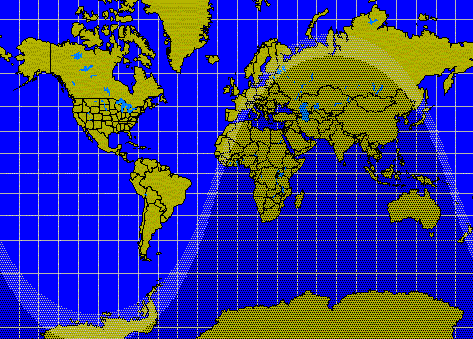
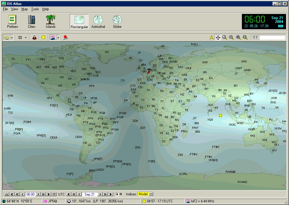
Radiation
pattern of a 1/2l antenna superposed on an
azimuthal equidistant map. Created by
LX4SKY with AC6LA's MultiProp. |
There
is another type of map which I find most helpful in my propagation
work, the azimuthal equidistant projection like the one displayed at
left, somewhat enhanced. You see that type of map in the back of the ARRL Operating
Manual, with the first one centered on W1AW. In contrast to the Mercator projection, where distortions
increase in going toward the poles, the azimuthal equidistant map is
centered on one point and the distortions increase with distance
toward the antipodal point on the opposite side of the earth. In fact, the antipodal point is distorted into a circle, in
contrast to the straight lines for the geographic poles in the
Mercator projection.
The
advantage of the azimuthal equidistant map is that all great-circle
paths going out from a QTH in the center are given by straight lines.
In addition, the
distance along the path is linear, out to the antipodal distance of
20,000 km. But the disadvantage of the azimuthal equidistant map is that
it has to be created for each QTH.
There
is another projection in which ALL great circles are straight lines,
no matter where on the map. That
is the gnomonic projection, used occasionally in propagation work.
The gnomonic projection is centered on one geographic pole or
the other and its disadvantage is non-linearity, with distortions
which increase in going to lower latitudes and the maps usually only
cover 30-45 degrees of latitude going equatorward from the poles.
Myself,
I prefer the azimuthal equidistant projection in the DXAID program
as it includes auroral zones based on the model used to display the
NOAA auroral maps on the Internet. The NOAA auroral maps on the Internet are given in terms of
auroral activity while the maps in DXAID use K-indices for the
corresponding levels of magnetic activity. So in using it, one can tell whether a path is more
tangential to the auroral zone, for a given level of magnetic
activity, or actually passes across the polar cap. With that kind of knowledge, one understands conditions far
better just on hearing a signal.
In
spite of that preference for propagation purposes, I have to admit
that I find the shape and motions of the terminator a bit odd in the
azimuthal equidistant map projection, something that I have a hard
time getting used to. In
contrast to that, I have no problem with the terminator in the
Mercator projection, its changes with time seem quite natural. So I have to say that each projection has its function as
well as virtues and that one really needs a familiarity with both to
deal with propagation problems.
Having
said all of that, we have to move on, above the E-region and into
ionization that's largely responsible for propagation, toward the
F-region peak. That
will take us right into the matter of propagation predictions by
bands, from fundamentals as well as computer programs.
Of
course, I've already made the point that a full-service propagation
program would include noise, say as signal/noise ratios. Now, I think you can understand it when I say a person
interested in propagation cannot get along without a good mapping
program. In the ideal
case, both the forecasting and mapping programs would be on the same
computer disk. Failing that, at least both ought to be readily available to
a DXer.
Reference
Notes
The
MINIPROP PLUS program by W6EL has been available for some years as a
DOS program and is now available for Windows 16 and 32 bit under the
name W6ELProp. The Mercator projection maps in this program are extremely
agile and fast, making it easy to make rapid comparisons of paths in
time. Today, there are however programs much more accurate on the
market.
DXAID
for example (now discontinued) had excellent graphics, particularly
the azimuthal equidistant mapping version with auroral zones
included. It also included a
propagation module based on the F-layer algorithm due to
Raymond Fricker of the BBC. However, like always in computing,
the auroral oval calculated by DXAID was outmoded and it was
advantageously replaced by the one provided by DXAtlas,
one of the seldom application that matches exactly the auroral oval
prediction calculated by SEC/NOAA.
|
|
|
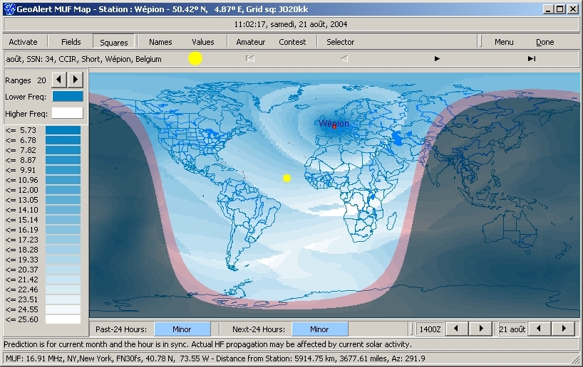
MUF map calculated by the VOACAP engine provided with GeoAlert-Extreme
from Kangaroo Tabor Software. |
All
these programs and algorithms are of course regularly improved, making
them more comparable to predictions that would be obtained from the
International Reference Ionosphere. Earlier tests for example made
in the '80s, show that Fricker's work, in MINIPROP and other
programs, comes closer to mimicing propagation predictions by IONCAP
than other programs available at the time. Today VOACAP predictions
are still better, and some applications even rely on real-time
ionospheric soundings.
Note
by LX4SKY. Today, among the best (I mean accurate and
flexible) propagation prediction programs available name VOACAP
Online and DXAtlas
(WinCAP
Wizard 3 and GeoAlert-Extreme
Wizard being no more available).
The
ultimate test of paths is found in ray-tracing, and the PropLab Pro
program from Solar Terrestrial Dispatch is the only one that is
presently available. The program not only traces propagation paths but also provides details
on the distribution of electrons, globally or vertically, and gives
a foundation for all ionospheric work. Myself, I would be absolutely LOST without PropLab Pro.
Ionization
of the E and F regions
Now
we have to get down to cases, dealing with the ionosphere above the
D- and E-regions. But
the transition is a smooth one, going from a well-mixed region
largely made up of molecules and molecular ions to a region where
collisions are less frequent, atoms become more abundant and
constituents start to be sorted out by their chemical weight. We'll never really get up to the case where hydrogen is the
dominant constituent but that is the idea, gravitational separation,
in the upper reaches above us.
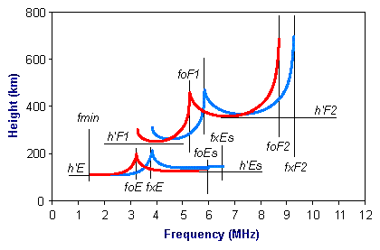
The
ionization in the E-region is under solar control and was shown by
the critical frequency depending on solar zenith angle (Z). Now, in
going higher, toward the F-region peak, solar control does continue,
up to the F1-region at about 200 km altitude. So the critical frequency foF1 during daytime is expressed
similarly:
foF1
(MHz) = [4.3 + 0.01 x SSN].[cos(Z)]0.2
|
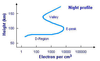
|
|
Peak
and valley in the E-region.
|
As
shown earlier, the electron density in the F1 region is greater than
the E-region and the same is true of the critical frequency. And
constant frequency contours will be centered about the sub-solar
point. But at large
zenith angles, the algorithm is less reliable and at night, the
ionization in the F1-region decreases to low values. It does not go to down to a vanishing level but, instead,
there is a "valley" in the electron density above the
night-time E-region, as shown at right.
The
origin of the valley is complex, related to the change from
molecular ions of oxygen and nitrogen down low to the appearance of
atomic oxygen and the ion-atom interchange above 90 km that produces
the molecular ion of nitric oxice (NO). Again, the ionization in darkness has the same origin as the
E-region.
Whether
day or night, the ionization in the D-region is just not great
enough to significantly bend or refract HF signals. On the other hand, during the day, ionization in the E-region
can cut off signals from reaching the F-region. In short, signals like that go off on low-angle, shorter
E-hops during the day.
At
night, HF signals will just pass through the weak ionization that
remains in the E-region, shown above, just as if it were not there. That's another way of saying that the night-time value for
foE is very low, even less than 0.5 MHz, and the region is no
impediment to the advance of HF signals. On the other hand, that's NOT the case for signals in the 160
meter band. That will
be VERY interesting but let's do some other things first.
|

|
|
Variation
of the plasma frequency with the sunspot number. |
For
example, let's look at how critical frequencies vary with sunspot
number so we can put effects of the various ionospheric regions in
perspective. For one
thing, with the different heights for the regions, E-region around
100 km while the F1-region is around 200 km and the F2-peak up
around 300 km, the frequency data will show how signals penetrate
into the ionization overhead. That has a bearing on the lengths of
the hops that result or, in more meaningful terms, on our ability to
work DX on the various bands. So let's look at a crude representation
of some mid-latitude critical frequency data for daytime conditions.
This graphic requires that you use your mind's eye to make
connections between data points but the results is pretty clear: the
lower E- and F1-regions which are under solar control show only
modest changes in critical frequency or electron density as the
sunspot number increases with solar activity.
The F-region, on the other hand, shows large changes in
critical frequency and is not under solar control, without any
simple algorithm involving the solar zenith angle like the E- and
F1-regions.
The
best way to illustrate the difference between solar control of the
E-region and the situation with the F-region is through the use of
maps showing the iso-frequency contours for the two regions.
|

|
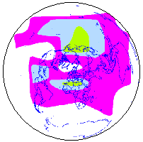
|
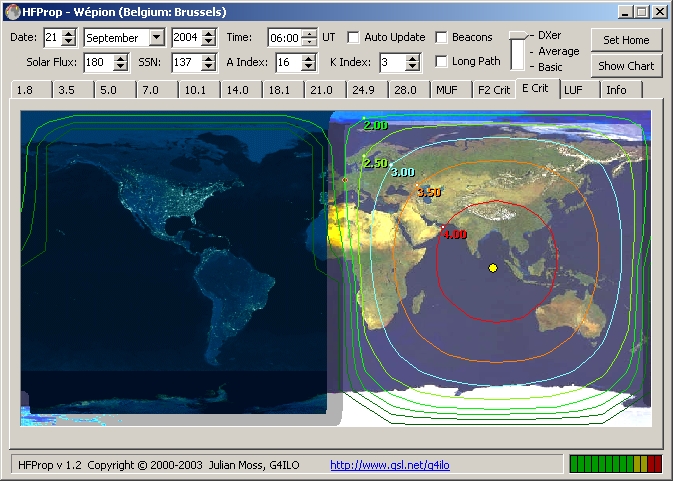
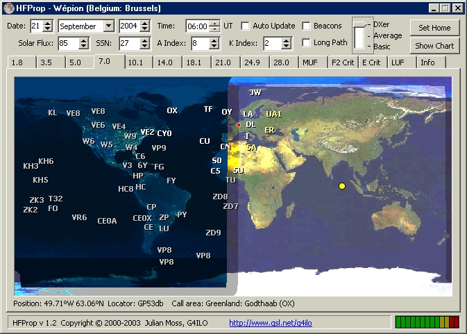
E-region
iso-frequency contours at fall equinox at 0600 UTC. |
So the map
displayed at right and generated with HFProp illustrates the situation for 0600 UTC on
the fall equinox. Of course, the sun is on the equator and at this time, it is located at
90° E longitude. The iso-frequency contours are centered on
the sub-solar point (but distorted by the Mercator projection).
Accordingly,
the left side of the figure is in darkness, and the
right side is in the sunlit portion of the earth, and the terminator,
the grayline, consists of two straight lines at 0° E and 180° E longitude.
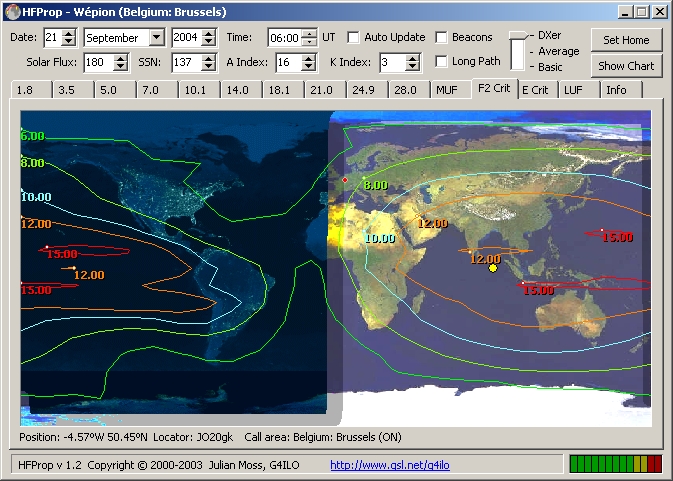
As
noted above, the situation is similar for the F1-region (or F2)
except that the critical frequencies are somewhat higher as shows
very well the map displayed below right.
But the idea of solar control is
clear from the E map at right; the ionization is where the sun shines and
essentially nothing in darkness!
Now
as far as the F-region is concerned, its peak is up around the 300
km level and depends on the season, time of day and sunspot number.
But at those heights, the electron collision frequency is low and
the recombination rate of electrons with the positive ions (O2+
and NO+) is quite low. So as shows very well the maps
displayed below, ionization continues to exist after sunset; the
geomagnetic control of the ionosphere is shown by the fact that the
F-region map for critical frequency foF2 is organized better by
geomagnetic coordinates rather than the usual geographical
coordinates.
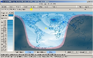
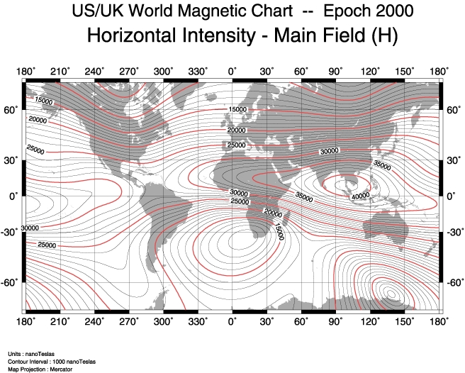
The
map below left conveys how the shape of geomagnetic dip equator compares with the
iso-frequency contour of the F2-region at low latitudes displayed at
right. The sunlit and dark hemispheres are the same as before but it is seen
that F-region continues after sunset, particularly at low latitudes
and along the direction of the geomagnetic dip equator.
 |
 |
|
At
left, dip of the geomagnetic equator at fall equinox at 0600 UTC predicted by
DXAtlas. At right, the
F2-critical frequency in the same conditions.
To compare with the E-region critical frequency (cf above
right). Note than on the side plunge into darkness
(left half) the propagation is still open for DX activities, mainly on
low
bands. The propagation is controlled (in quiet time) by the horizontal
component of the geomagnetic field and in a much lesser extent by the
sun ionization. |
|
Such
critical frequency maps demonstrate that the ionosphere is
controlled by the geomagnetic field at great heights but down lower,
the distribution of ionization is under solar control. The transition occurs in going up through the
F1-region. As for DX propagation, it is controlled in quiet times by the
geomagnetic field but it doesn't take much imagination to think that
any sort of disturbance of the field would upset DXing. More later!
Reference
Notes
Critical
frequency maps of the E- and F-regions can be seen in my book The
Little Pistol's Guide to HF Propagation. In
addition, they will be found in books Radio Amateurs Guide to
the Ionosphere by McNamara, and Ionospheric
Radio (IEE Electromagnetic Waves Series, Vol. 31) by K.Davies.
Excellent
critical frequency maps are obtained from the PropLab Pro
program. In fact, that program gives a full complement of ionospheric
maps and in several projections.
Next
chapter
Down-Sizing of the Ionosphere


